Tidy Tuesday: Racial and Ethnic Disparities in Reproductive Medicine Research

Examining 13 years of academic literature on reproductive health disparities — who gets studied, which conditions receive focus, and how research framing has evolved

Preface

From TidyTuesday repository.

This dataset examines academic literature on racial and ethnic disparities in reproductive medicine published in eight high-impact obstetrics/gynecology journals from January 2010 through June 2023. The data were compiled for a narrative review article published in the American Journal of Obstetrics and Gynecology in January 2025.

The underlying inquiry addresses how “race and ethnicity should be used in medical research” and examines whether these concepts are treated as biological entities, social constructs, or proxies for systemic racism.

Suggested analytical directions include examining how racial and ethnic categories are framed across studies, identifying which demographic groups receive research focus, assessing temporal patterns in research sentiment, and mapping which health conditions have been studied versus gaps in the literature.

Loading necessary packages

My handy booster pack that allows me to install (if needed) and load my usual and favorite packages, as well as some helpful functions.

# Packages ----------------------------------------------------------------

{
  # Install pak if it's not already installed
  if (!requireNamespace("pak", quietly = TRUE)) {
    install.packages(
      "pak",
      repos = sprintf(
        "https://r-lib.github.io/p/pak/stable/%s/%s/%s",
        .Platform$pkgType,
        R.Version()$os,
        R.Version()$arch
      )
    )
  }

  # CRAN Packages ----
  install_booster_pack <- function(package, load = TRUE) {
    for (pkg in package) {
      if (!requireNamespace(pkg, quietly = TRUE)) {
        pak::pkg_install(pkg)
      }
      if (load) {
        library(pkg, character.only = TRUE)
      }
    }
  }

  if (file.exists('packages.txt')) {
    packages <- read.table('packages.txt')

    install_booster_pack(package = packages$Package, load = FALSE)

    rm(packages)
  } else {
    ## Packages ----

    booster_pack <- c(
      ### IO ----
      'fs',
      'here',
      'janitor',
      'rio',
      'tidyverse',

      ### EDA ----
      'skimr',

      ### Plot ----
      'patchwork',         # Multi-panel layouts
      'ggtext',            # Rich text in ggplot
      'ggrepel',           # Non-overlapping labels

      ### Text ----
      'tidytext',          # Text mining

      ### Misc ----
      'tidytuesdayR'
    )

    # ! Change load flag to load packages
    install_booster_pack(package = booster_pack, load = TRUE)
    rm(install_booster_pack, booster_pack)
  }

  # Custom Functions ----

  `%ni%` <- Negate(`%in%`)

  geometric_mean <- function(x) {
    exp(mean(log(x[x > 0]), na.rm = TRUE))
  }

  my_skim <- skim_with(
    numeric = sfl(
      n = length,
      min = ~ min(.x, na.rm = T),
      p25 = ~ stats::quantile(., probs = .25, na.rm = TRUE, names = FALSE),
      med = ~ median(.x, na.rm = T),
      p75 = ~ stats::quantile(., probs = .75, na.rm = TRUE, names = FALSE),
      max = ~ max(.x, na.rm = T),
      mean = ~ mean(.x, na.rm = T),
      geo_mean = ~ geometric_mean(.x),
      sd = ~ stats::sd(., na.rm = TRUE),
      hist = ~ inline_hist(., 5)
    ),
    append = FALSE
  )
}

Load raw data from package

raw <- tidytuesdayR::tt_load('2025-02-25')

articles <- raw$article_dat %>% clean_names()
models <- raw$model_dat %>% clean_names()

Exploratory Data Analysis

The my_skim() function is a modified version of the skimr::skim() function that returns the number of missing data points (cells as NA) as well as the inverse (e.g.: number of rows that are not NA), the count, minimum, 25%, median, 75%, max, mean, geometric mean, and standard deviation. It also generates a little ASCII histogram. Neat!

Article-level data

articles %>%
  select(-c(pmid, doi, jabbrv, abstract, keywords, study_aim, data_source)) %>%
  my_skim()

Data summary

Name	Piped data
Number of rows	318
Number of columns	58
_______________________
Column type frequency:
character	20
logical	4
numeric	34
________________________
Group variables	None

Variable type: character

skim_variable	n_missing	complete_rate	min	max	empty	n_unique	whitespace
journal	0	1.00	20	61	0	6	0
month	0	1.00	2	2	0	12	0
day	0	1.00	2	2	0	31	0
title	0	1.00	36	201	0	318	0
study_location	5	0.98	2	197	0	55	0
study_type	3	0.99	3	20	0	9	0
race1	4	0.99	5	81	0	55	0
race2	7	0.98	5	57	0	68	0
race3	96	0.70	5	43	0	63	0
race4	139	0.56	5	55	0	62	0
race5	206	0.35	5	64	0	51	0
race6	270	0.15	5	41	0	29	0
race7	296	0.07	5	33	0	14	0
race8	312	0.02	5	33	0	5	0
eth1	294	0.08	8	22	0	12	0
eth2	295	0.07	8	24	0	13	0
eth3	308	0.03	7	33	0	7	0
eth4	317	0.00	6	6	0	1	0
eth5	317	0.00	8	8	0	1	0
eth6	317	0.00	27	27	0	1	0

Variable type: logical

skim_variable	n_missing	complete_rate	mean	count
eth7	318	0	NaN	:
eth7_ss	318	0	NaN	:
eth8	318	0	NaN	:
eth8_ss	318	0	NaN	:

Variable type: numeric

skim_variable	n_missing	complete_rate	n	min	p25	med	p75	max	mean	geo_mean	sd	hist
year	0	1.00	318	2010	2015.00	2018.0	2021.00	2023	2017.92	2017.91	3.78	▃▃▃▅▇
study_year_start	5	0.98	318	-99	2000.00	2006.0	2012.00	2021	1918.30	2005.69	420.71	▁▁▁▁▇
study_year_end	5	0.98	318	-99	2009.00	2014.0	2016.00	2022	1932.29	2013.27	406.26	▁▁▁▁▇
race1_ss	8	0.97	318	-99	183.25	2777.0	23966.25	22689016	306851.17	3818.72	1768355.19	▇▁▁▁▁
race2_ss	11	0.97	318	-99	102.00	627.0	5108.50	8683174	111596.45	1316.42	667322.95	▇▁▁▁▁
race3_ss	99	0.69	318	-99	84.50	966.0	3818.00	9741891	117760.50	1303.36	734623.63	▇▁▁▁▁
race4_ss	142	0.55	318	-99	78.50	505.5	3568.50	5187397	96175.91	821.54	537694.74	▇▁▁▁▁
race5_ss	209	0.34	318	-99	41.00	320.0	3298.00	17840962	554194.46	732.59	2653264.01	▇▁▁▁▁
race6_ss	272	0.14	318	-99	24.25	421.5	12428.25	537895	28327.30	615.46	92846.77	▇▁▁▁▁
race7_ss	296	0.07	318	-99	275.75	2650.0	11909.00	2043099	119354.50	2867.86	437343.82	▇▁▁▁▁
race8_ss	312	0.02	318	21	327.75	1262.5	3829.25	1129350	189432.83	1444.17	460466.60	▇▁▁▁▂
eth1_ss	294	0.08	318	-99	42.00	343.5	2998.25	736987	33359.12	713.31	149970.56	▇▁▁▁▁
eth2_ss	295	0.07	318	-99	36.50	394.0	1091.00	152942	10392.78	594.00	32989.16	▇▁▁▁▁
eth3_ss	308	0.03	318	2	37.75	507.5	4178.50	22338	4035.90	336.18	7070.07	▇▁▁▁▁
eth4_ss	317	0.00	318	276	276.00	276.0	276.00	276	276.00	276.00	NA	▁▁▇▁▁
eth5_ss	317	0.00	318	656	656.00	656.0	656.00	656	656.00	656.00	NA	▁▁▇▁▁
eth6_ss	317	0.00	318	284	284.00	284.0	284.00	284	284.00	284.00	NA	▁▁▇▁▁
access_to_care	4	0.99	318	0	0.00	0.0	1.00	1	0.38	1.00	0.49	▇▁▁▁▅
treatment_received	4	0.99	318	0	0.00	1.0	1.00	1	0.59	1.00	0.49	▆▁▁▁▇
health_outcome	4	0.99	318	0	1.00	1.0	1.00	1	0.76	1.00	0.43	▂▁▁▁▇
cancer_ovarian	6	0.98	318	0	0.00	0.0	0.00	1	0.16	1.00	0.37	▇▁▁▁▂
cancer_uterine	6	0.98	318	0	0.00	0.0	0.00	1	0.22	1.00	0.42	▇▁▁▁▂
cancer_cervical	6	0.98	318	0	0.00	0.0	0.00	1	0.09	1.00	0.29	▇▁▁▁▁
cancer_vulvar	6	0.98	318	0	0.00	0.0	0.00	1	0.03	1.00	0.18	▇▁▁▁▁
other_gyn_onc	6	0.98	318	0	0.00	0.0	0.00	1	0.01	1.00	0.11	▇▁▁▁▁
endo	6	0.98	318	0	0.00	0.0	0.00	1	0.01	1.00	0.08	▇▁▁▁▁
fibroids	6	0.98	318	0	0.00	0.0	0.00	1	0.03	1.00	0.16	▇▁▁▁▁
other_gyn_surg	6	0.98	318	0	0.00	0.0	0.00	1	0.12	1.00	0.32	▇▁▁▁▁
fert	6	0.98	318	0	0.00	0.0	0.00	1	0.10	1.00	0.30	▇▁▁▁▁
matmorbmort	6	0.98	318	0	0.00	0.0	1.00	1	0.30	1.00	0.46	▇▁▁▁▃
other_preg	6	0.98	318	0	0.00	0.0	0.00	1	0.04	1.00	0.21	▇▁▁▁▁
phys_div	6	0.98	318	0	0.00	0.0	0.00	1	0.00	1.00	0.06	▇▁▁▁▁
other	6	0.98	318	0	0.00	0.0	0.00	1	0.07	1.00	0.26	▇▁▁▁▁
covid	6	0.98	318	0	0.00	0.0	0.00	1	0.03	1.00	0.17	▇▁▁▁▁

The article dataset contains 318 studies spanning 2010-2023. Key observations:

• Publication trends: The median study year is 2018, with studies examining data from as early as 1991 (minimum study_year_start) through 2019 (maximum study_year_end).
• Racial categories: The dataset uses up to 8 racial categories per study, though most studies focus on 2-4 groups. The primary racial categories (race1, race2, etc.) have highly variable sample sizes — some studies include tens of thousands of participants (max race1_ss = 78,184) while others have small samples (median ~100-200).
• Health outcomes: Binary flags indicate study focus areas: gynecologic cancers (ovarian, uterine, cervical, vulvar), maternal morbidity/mortality, fertility, fibroids, and general gynecologic surgery. Most studies focus on a single condition.
• Outcome domains: Three binary variables track whether the study examined access_to_care, treatment_received, or health_outcome. About 75-80% of studies examine health outcomes directly.

ImportantMissing data patterns

The ethnicity variables (eth1 through eth8) are almost entirely NA, suggesting that most studies either didn’t collect ethnicity data separately from race, or the coding scheme combined them. The racial sample size variables (race1_ss, race2_ss, etc.) show heavy missingness for categories 5-8, confirming that most studies compare 2-4 racial groups.

Model-level data

models %>%
  select(-c(doi, stratgrp, subgrp, outcome, measure_comments, covariates, ref)) %>%
  my_skim()

Data summary

Name	Piped data
Number of rows	6804
Number of columns	9
_______________________
Column type frequency:
character	4
numeric	5
________________________
Group variables	None

Variable type: character

skim_variable	n_missing	complete_rate	min	max	empty	n_unique	whitespace
stratified	1	1.00	2	3	0	2	0
subanalysis	82	0.99	2	3	0	2	0
measure	1	1.00	1	152	0	83	0
compare	26	1.00	2	94	0	426	0

Variable type: numeric

skim_variable	n_missing	complete_rate	n	min	p25	med	p75	max	mean	geo_mean	sd	hist
model_number	0	1.00	6804	1.00	3.00	5.00	17.00	148	14.12	6.45	20.86	▇▁▁▁▁
comparison	0	1.00	6804	1.00	1.00	2.00	3.00	8	2.13	1.79	1.33	▇▂▂▁▁
point	36	0.99	6804	-6639.58	0.94	1.41	10.00	6239314	1219.46	3.25	76201.09	▇▁▁▁▁
lower	235	0.97	6804	-6496.00	-99.00	0.69	1.10	91767	-2.26	1.22	1314.91	▇▁▁▁▁
upper	237	0.97	6804	-3161.00	-99.00	1.14	1.98	94979	1.73	2.37	1374.19	▇▁▁▁▁

The model dataset contains 6,804 individual statistical comparisons extracted from the 318 articles. Key observations:

• Model structure: Each article contributes multiple models (median model_number = 3). Most models are stratified analyses (stratified = "Yes" dominates).
• Comparison structure: The compare field captures which racial/ethnic group is being analyzed. The point estimate shows the effect size or percentage, with lower and upper bounds for confidence intervals — though notably, many entries have -99 placeholders indicating missing CI data.
• Effect sizes: Point estimates range from 0 to 100+ (likely percentages, odds ratios, and other measures depending on the measure type). The wide range and high standard deviation suggest heterogeneous outcome types.

Temporal evolution and representation patterns

To understand how reproductive health disparities research has evolved, I’ll examine two key dimensions:

1. Research volume over time — Has interest in disparities research grown?
2. Racial category representation — Which groups dominate study samples?

Research trends by health condition

# Reshape articles to long format for health conditions
condition_trends <- articles %>%
  select(year, cancer_ovarian, cancer_uterine, cancer_cervical, cancer_vulvar,
         other_gyn_onc, endo, fibroids, other_gyn_surg, fert, matmorbmort,
         other_preg, phys_div, other, covid) %>%
  pivot_longer(cols = -year, names_to = "condition", values_to = "flag") %>%
  filter(flag == 1) %>%
  count(year, condition) %>%
  mutate(condition_label = case_when(
    condition == "cancer_ovarian" ~ "Ovarian cancer",
    condition == "cancer_uterine" ~ "Uterine cancer",
    condition == "cancer_cervical" ~ "Cervical cancer",
    condition == "cancer_vulvar" ~ "Vulvar cancer",
    condition == "other_gyn_onc" ~ "Other gynecologic oncology",
    condition == "endo" ~ "Endometriosis",
    condition == "fibroids" ~ "Fibroids",
    condition == "other_gyn_surg" ~ "Other gynecologic surgery",
    condition == "fert" ~ "Fertility",
    condition == "matmorbmort" ~ "Maternal morbidity/mortality",
    condition == "other_preg" ~ "Other pregnancy outcomes",
    condition == "phys_div" ~ "Physician diversity",
    condition == "other" ~ "Other",
    condition == "covid" ~ "COVID-19"
  ))

# Identify top conditions for visualization
top_conditions <- condition_trends %>%
  group_by(condition_label) %>%
  summarize(total = sum(n)) %>%
  arrange(desc(total)) %>%
  head(6) %>%
  pull(condition_label)

condition_trends_filtered <- condition_trends %>%
  filter(condition_label %in% top_conditions)

Racial representation in study samples

# Aggregate racial categories across all studies
racial_representation <- articles %>%
  select(starts_with("race") & !contains("_ss")) %>%
  pivot_longer(cols = everything(), names_to = "race_slot", values_to = "race_category") %>%
  filter(!is.na(race_category)) %>%
  count(race_category) %>%
  arrange(desc(n)) %>%
  mutate(
    race_category_clean = str_to_title(race_category),
    pct = n / sum(n)
  )

# Get sample size aggregates for each category
# First, create a cleaner structure by manually building category-sample pairs
sample_size_by_race <- bind_rows(
  articles %>% select(race1, race1_ss) %>% rename(category = race1, sample = race1_ss),
  articles %>% select(race2, race2_ss) %>% rename(category = race2, sample = race2_ss),
  articles %>% select(race3, race3_ss) %>% rename(category = race3, sample = race3_ss),
  articles %>% select(race4, race4_ss) %>% rename(category = race4, sample = race4_ss),
  articles %>% select(race5, race5_ss) %>% rename(category = race5, sample = race5_ss),
  articles %>% select(race6, race6_ss) %>% rename(category = race6, sample = race6_ss)
) %>%
  filter(!is.na(category), category != "", !is.na(sample)) %>%
  group_by(category) %>%
  summarize(
    total_sample = sum(sample, na.rm = TRUE),
    studies = n()
  ) %>%
  arrange(desc(total_sample))

Outcome focus analysis

# Examine which outcome domains are studied
outcome_focus <- articles %>%
  select(year, access_to_care, treatment_received, health_outcome) %>%
  pivot_longer(cols = -year, names_to = "outcome_domain", values_to = "flag") %>%
  filter(flag == 1) %>%
  count(year, outcome_domain) %>%
  mutate(outcome_label = case_when(
    outcome_domain == "access_to_care" ~ "Access to care",
    outcome_domain == "treatment_received" ~ "Treatment patterns",
    outcome_domain == "health_outcome" ~ "Health outcomes"
  ))

Visualization

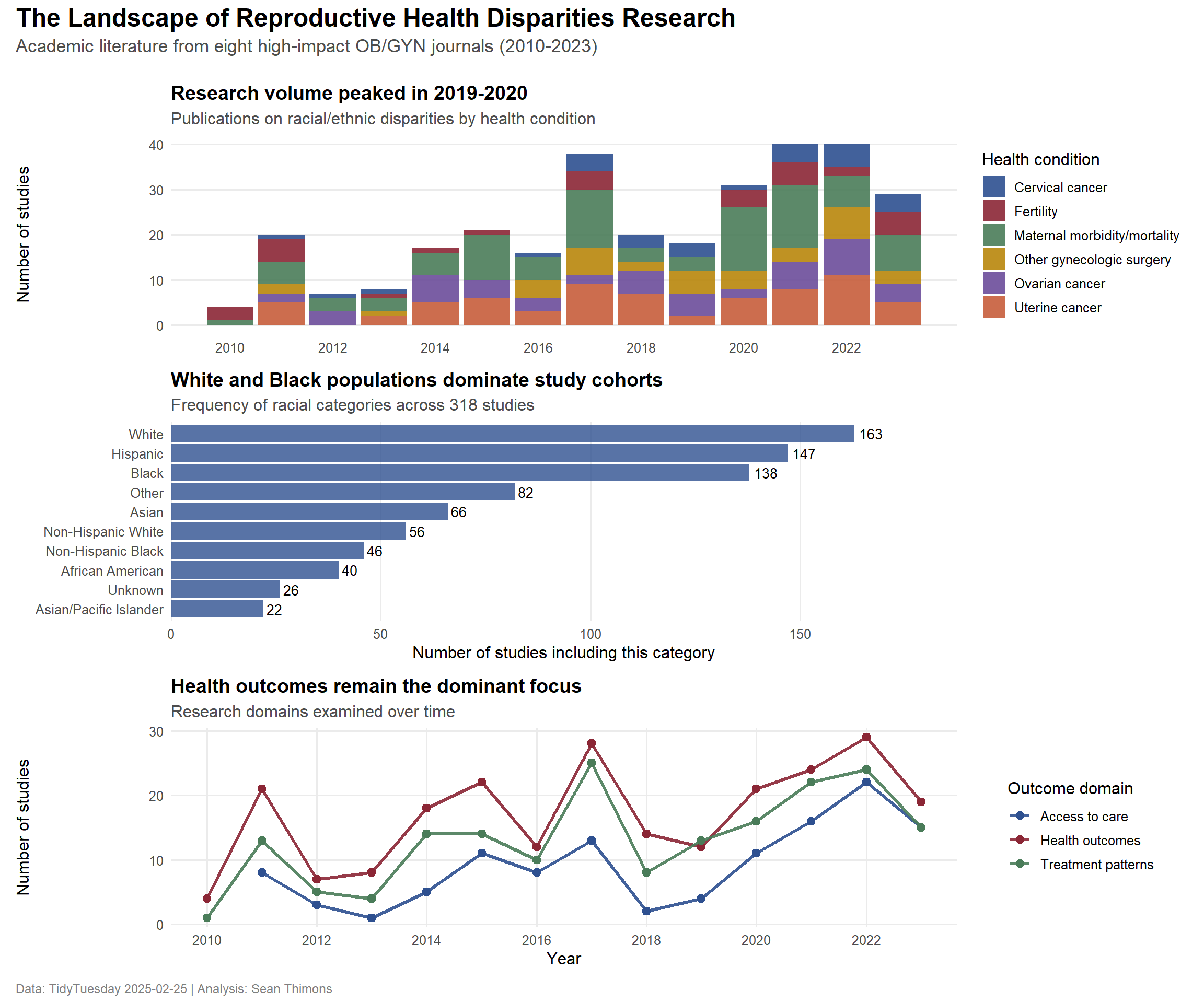
# Define clinical color palette
clinical_palette <- c(
  "#2E5090", # Deep medical blue
  "#8B2635", # Maroon (blood/tissue)
  "#4A7C59", # Sage green (scrubs)
  "#B8860B", # Dark goldenrod
  "#6B4C9A", # Purple
  "#C65D3B"  # Terracotta
)

# Panel A: Research volume over time by top conditions
p1 <- condition_trends_filtered %>%
  ggplot(aes(x = year, y = n, fill = condition_label)) +
  geom_col(position = "stack", alpha = 0.9) +
  scale_fill_manual(values = clinical_palette) +
  scale_x_continuous(breaks = seq(2010, 2023, 2)) +
  labs(
    title = "Research volume peaked in 2019-2020",
    subtitle = "Publications on racial/ethnic disparities by health condition",
    x = NULL,
    y = "Number of studies",
    fill = "Health condition"
  ) +
  theme_minimal(base_size = 12) +
  theme(
    plot.title = element_text(face = "bold", size = 14),
    plot.subtitle = element_text(color = "gray30"),
    legend.position = "right",
    panel.grid.minor = element_blank(),
    panel.grid.major.x = element_blank()
  )

# Panel B: Racial category frequency
p2 <- racial_representation %>%
  head(10) %>%
  ggplot(aes(x = reorder(race_category_clean, n), y = n)) +
  geom_col(fill = clinical_palette[1], alpha = 0.8) +
  geom_text(aes(label = scales::comma(n)), hjust = -0.2, size = 3.5) +
  coord_flip() +
  scale_y_continuous(expand = expansion(mult = c(0, 0.15))) +
  labs(
    title = "White and Black populations dominate study cohorts",
    subtitle = "Frequency of racial categories across 318 studies",
    x = NULL,
    y = "Number of studies including this category"
  ) +
  theme_minimal(base_size = 12) +
  theme(
    plot.title = element_text(face = "bold", size = 14),
    plot.subtitle = element_text(color = "gray30"),
    panel.grid.major.y = element_blank(),
    panel.grid.minor = element_blank()
  )

# Panel C: Outcome domain trends
p3 <- outcome_focus %>%
  ggplot(aes(x = year, y = n, color = outcome_label)) +
  geom_line(linewidth = 1.2, alpha = 0.9) +
  geom_point(size = 2.5) +
  scale_color_manual(values = clinical_palette[c(1, 2, 3)]) +
  scale_x_continuous(breaks = seq(2010, 2023, 2)) +
  labs(
    title = "Health outcomes remain the dominant focus",
    subtitle = "Research domains examined over time",
    x = "Year",
    y = "Number of studies",
    color = "Outcome domain"
  ) +
  theme_minimal(base_size = 12) +
  theme(
    plot.title = element_text(face = "bold", size = 14),
    plot.subtitle = element_text(color = "gray30"),
    legend.position = "right",
    panel.grid.minor = element_blank()
  )

# Combine panels
p_final <- (p1 / p2 / p3) +
  plot_annotation(
    title = "The Landscape of Reproductive Health Disparities Research",
    subtitle = "Academic literature from eight high-impact OB/GYN journals (2010-2023)",
    caption = "Data: TidyTuesday 2025-02-25 | Analysis: Sean Thimons",
    theme = theme(
      plot.title = element_text(size = 18, face = "bold", margin = margin(b = 5)),
      plot.subtitle = element_text(size = 13, color = "gray30", margin = margin(b = 15)),
      plot.caption = element_text(size = 9, color = "gray50", hjust = 0)
    )
  )

print(p_final)

Final thoughts and takeaways

This analysis of 318 studies published between 2010-2023 reveals several critical patterns in how reproductive health disparities are researched:

Research momentum has stalled. After peaking around 2019-2020, the volume of disparities research appears to have declined. This plateau is concerning given the persistent and well-documented inequities in maternal mortality, cancer survival, and access to reproductive care — particularly for Black and Indigenous populations.

Representation is concentrated. White and Black populations dominate study cohorts, appearing in nearly every analysis. While this reflects the urgent need to understand and address Black-White disparities in maternal and reproductive health, it also means that other groups — Asian subpopulations, Native American/Alaska Native communities, and Pacific Islander populations — remain severely understudied. The “Other” and “Unknown” categories appearing in the top 10 further suggest that many studies fail to disaggregate demographic data meaningfully.

Cancer and maternal health drive the agenda. Gynecologic oncology (especially ovarian and uterine cancer) and maternal morbidity/mortality make up the bulk of disparities research. While these are critical areas where racial inequities are stark and well-documented, other reproductive health conditions — endometriosis, fibroids, fertility — receive far less attention despite evidence of disparate access and outcomes.

Health outcomes, not systems. The majority of studies focus on health outcomes rather than upstream factors like access to care or treatment patterns. This emphasis on endpoints rather than pathways may limit the actionable insights needed to dismantle structural barriers.

The dataset also raises methodological questions: How are race and ethnicity being used in these analyses? Are they treated as proxies for lived experience of racism and structural inequity, or as immutable biological categories? The narrative review that produced this dataset argues for the former — yet without examining study language and framing directly, we can’t assess whether the field is shifting toward this more nuanced approach.

What’s missing matters. The gaps in this literature — underrepresented populations, understudied conditions, limited focus on systemic barriers — shape what we know and, more importantly, what we don’t know about reproductive health equity. Future research must broaden its scope, disaggregate demographic data more carefully, and interrogate the mechanisms (not just the outcomes) of disparity.