Where the Federal Workforce Lives

Mapping which counties have the highest share of federal employees using ACS 1-year estimates

Preface

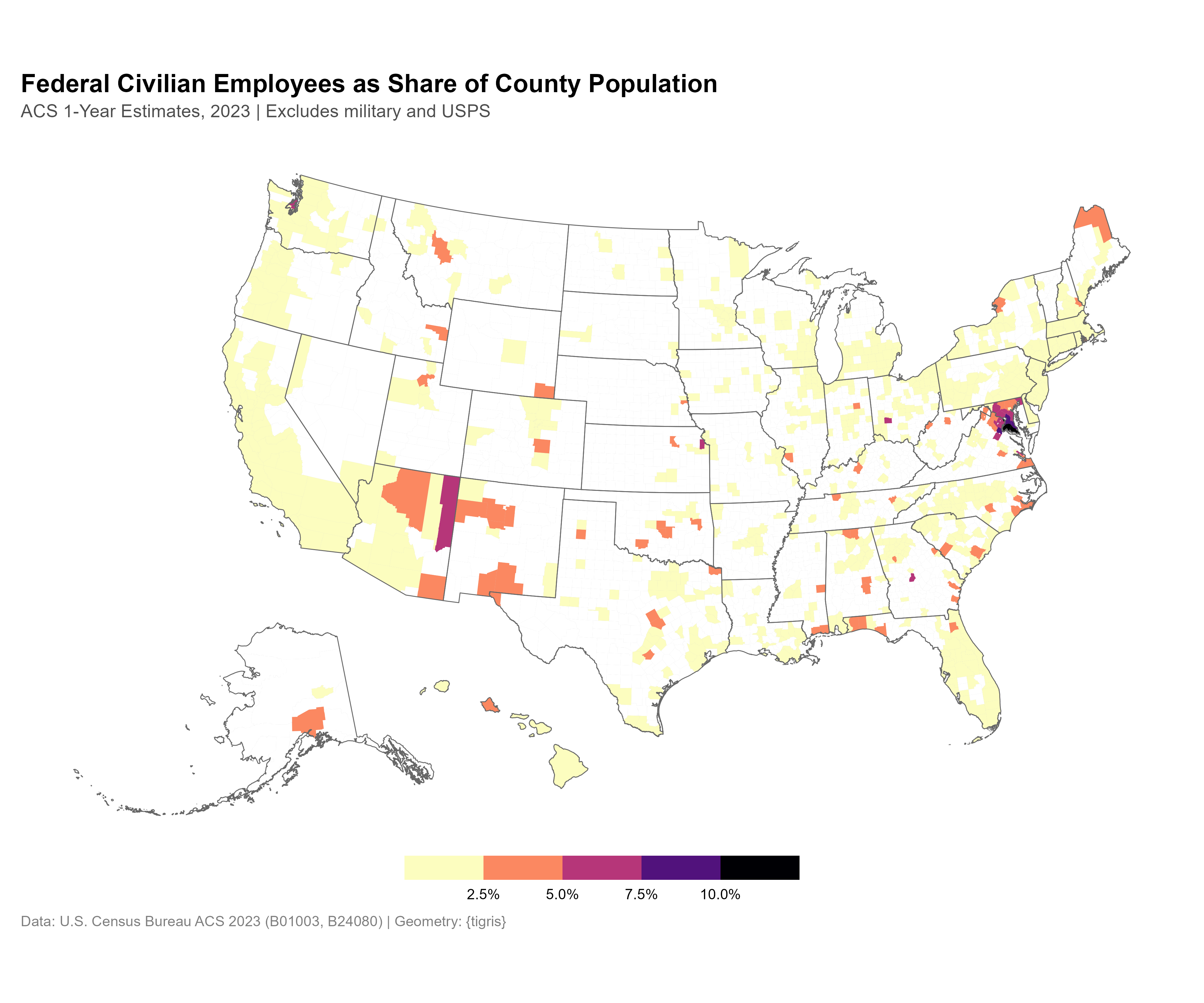
Where do federal government employees (excluding military personnel and USPS workers) make up the largest share of the 18+ labor force? Using the American Community Survey 1-year estimates for 2023, I pulled county-level data on federal employment and mapped the results.

The ACS variables used:

• B01003_001: Total population
• B24080_009: Male federal government workers (civilian)
• B24080_019: Female federal government workers (civilian)

Loading necessary packages

# Packages ----------------------------------------------------------------

{
  # Use Posit Package Manager for pre-built Linux binaries
  if (Sys.info()[["sysname"]] == "Linux") {
    distro <- system("lsb_release -cs", intern = TRUE)
    options(repos = c(CRAN = paste0(
      "https://packagemanager.posit.co/cran/__linux__/", distro, "/latest"
    )))
  }

  # Install pak if it's not already installed
  if (!requireNamespace("pak", quietly = TRUE)) {
    install.packages(
      "pak",
      repos = sprintf(
        "https://r-lib.github.io/p/pak/stable/%s/%s/%s",
        .Platform$pkgType,
        R.Version()$os,
        R.Version()$arch
      )
    )
  }

  # CRAN Packages ----
  install_booster_pack <- function(package, load = TRUE) {
    for (pkg in package) {
      if (!requireNamespace(pkg, quietly = TRUE)) {
        pak::pkg_install(pkg)
      }
      if (load) {
        library(pkg, character.only = TRUE)
      }
    }
  }

  booster_pack <- c(
    ### IO ----
    'fs',
    'here',
    'janitor',
    'rio',
    'tidyverse',

    ### EDA ----
    'skimr',

    ### Plot ----
    'paletteer',
    'ggtext',
    'ggrepel',
    'gghighlight',
    'ggforce',
    'geomtextpath',

    ### Geospatial ----
    'tidycensus',
    'tigris',
    'sf',

    ### Table ----
    'ggpubr',
    'patchwork'
  )

  install_booster_pack(package = booster_pack, load = TRUE)
  rm(install_booster_pack, booster_pack)

  # Custom Functions ----

  `%ni%` <- Negate(`%in%`)

  geometric_mean <- function(x) {
    exp(mean(log(x[x > 0]), na.rm = TRUE))
  }

  my_skim <- skim_with(
    numeric = sfl(
      n = length,
      min = ~ min(.x, na.rm = T),
      p25 = ~ stats::quantile(., probs = .25, na.rm = TRUE, names = FALSE),
      med = ~ median(.x, na.rm = T),
      p75 = ~ stats::quantile(., probs = .75, na.rm = TRUE, names = FALSE),
      max = ~ max(.x, na.rm = T),
      mean = ~ mean(.x, na.rm = T),
      geo_mean = ~ geometric_mean(.x),
      sd = ~ stats::sd(., na.rm = TRUE),
      hist = ~ inline_hist(., 5)
    ),
    append = FALSE
  )
}

Load data from ACS

raw <-
  get_acs(
    geography = "county",
    variables = c("B01003_001", "B24080_009", "B24080_019"),
    year = 2023,
    survey = "acs1",
    output = "wide",
    geometry = FALSE
  )

states <- tigris::states(year = 2023, cb = TRUE) %>%
  filter(STUSPS %in% state.abb) %>%
  shift_geometry()

counties <- tigris::counties(year = 2023, cb = TRUE) %>%
  filter(STATEFP %in% states$STATEFP) %>%
  shift_geometry()

Exploratory Data Analysis

Dataset Structure

cleaned <- raw %>%
  group_by(GEOID) %>%
  summarize(
    percentage = sum(B24080_009E, B24080_019E) / B01003_001E,
    pop_fed = sum(B24080_009E, B24080_019E),
    total = B01003_001E
  )

cat("Counties with ACS 1-yr data:", nrow(cleaned), "\n")

Counties with ACS 1-yr data: 854 

cat("Counties with federal employees:", sum(cleaned$pop_fed > 0, na.rm = TRUE), "\n")

Counties with federal employees: 854 

cat("Total federal employees captured:", scales::comma(sum(cleaned$pop_fed, na.rm = TRUE)), "\n")

Total federal employees captured: 3,832,310 

my_skim(cleaned %>% select(percentage, pop_fed, total))

Data summary

Name	cleaned %>% select(percen…
Number of rows	854
Number of columns	3
_______________________
Column type frequency:
numeric	3
________________________
Group variables	None

Variable type: numeric

skim_variable	n_missing	complete_rate	n	min	p25	med	p75	max	mean	geo_mean	sd	hist
percentage	0	1	854	0	0.01	0.01	0.02	0.12	0.01	0.01	0.01	▇▁▁▁▁
pop_fed	0	1	854	37	913.25	1958.00	4915.00	78810.00	4487.48	2087.22	8160.51	▇▁▁▁▁
total	0	1	854	63661	96742.00	163086.50	348316.75	9663345.00	337437.25	198699.64	577730.93	▇▁▁▁▁

NoteACS 1-Year Coverage

The ACS 1-year estimates only cover geographies with populations of 65,000+. This means smaller rural counties — some of which host significant federal installations — are excluded. The map will show gaps where data isn’t available, not where federal employees don’t exist.

Top Counties by Federal Workforce Share

cleaned_geo <- counties %>%
  left_join(cleaned, join_by(GEOID))

cleaned_geo %>%
  sf::st_drop_geometry() %>%
  select(STATE_NAME, NAME, percentage, pop_fed, total) %>%
  filter(!is.na(percentage)) %>%
  arrange(desc(percentage)) %>%
  head(15) %>%
  mutate(percentage = scales::percent(percentage, accuracy = 0.1)) %>%
  knitr::kable(
    col.names = c("State", "County", "Fed %", "Fed Employees", "Total Pop"),
    format.args = list(big.mark = ",")
  )

State	County	Fed %	Fed Employees	Total Pop
Virginia	Arlington	12.1%	28,356	234,162
Maryland	Charles	11.0%	18,929	171,973
Virginia	Alexandria	10.3%	15,916	155,230
Maryland	St. Mary’s	10.2%	11,716	115,281
Virginia	Stafford	9.8%	16,214	165,428
Maryland	Calvert	7.9%	7,443	94,728
Maryland	Prince George’s	7.7%	73,266	947,430
Maryland	Montgomery	7.1%	74,897	1,058,474
Virginia	Fairfax	6.9%	78,810	1,141,878
Washington	Kitsap	6.7%	18,482	277,658
Virginia	Spotsylvania	6.6%	9,843	149,588
Virginia	York	6.3%	4,435	70,952
Virginia	Prince William	6.2%	30,586	489,640
Kansas	Leavenworth	6.1%	5,115	83,518
Maryland	Anne Arundel	6.1%	36,069	594,582

Top States by Federal Workforce Share

cleaned_geo %>%
  sf::st_drop_geometry() %>%
  filter(!is.na(percentage)) %>%
  group_by(STATE_NAME) %>%
  summarize(
    st_percent = sum(pop_fed, na.rm = TRUE) / sum(total, na.rm = TRUE),
    total_fed = sum(pop_fed, na.rm = TRUE),
    .groups = "drop"
  ) %>%
  arrange(desc(st_percent)) %>%
  head(10) %>%
  mutate(st_percent = scales::percent(st_percent, accuracy = 0.1)) %>%
  knitr::kable(
    col.names = c("State", "Fed %", "Total Fed Employees"),
    format.args = list(big.mark = ",")
  )

State	Fed %	Total Fed Employees
Maryland	5.5%	324,254
Virginia	4.7%	297,957
Alaska	3.3%	16,531
Hawaii	3.0%	42,593
New Mexico	2.9%	47,143
Wyoming	2.4%	4,314
West Virginia	2.3%	16,687
Oklahoma	2.2%	57,636
Alabama	1.9%	72,382
Mississippi	1.8%	25,000

ImportantThe Beltway Effect

The D.C. metro area dominates, but the geographic spread beyond that tells the more interesting story — military-adjacent counties, land management hubs, and research corridors all show elevated federal presence. The federal workforce isn’t just a Beltway phenomenon.

Visualization

hero <- ggplot() +
  geom_sf(
    data = counties,
    fill = "grey95",
    color = "grey80",
    linewidth = 0.1
  ) +
  geom_sf(
    data = cleaned_geo,
    mapping = aes(fill = percentage),
    color = NA
  ) +
  geom_sf(
    data = states,
    fill = NA,
    color = "grey40",
    linewidth = 0.3
  ) +
  scale_fill_viridis_b(
    name = NULL,
    option = 'magma',
    na.value = "white",
    n.breaks = 6,
    direction = -1,
    labels = scales::label_percent()
  ) +
  labs(
    title = "Federal Civilian Employees as Share of County Population",
    subtitle = "ACS 1-Year Estimates, 2023 | Excludes military and USPS",
    caption = "Data: U.S. Census Bureau ACS 2023 (B01003, B24080) | Geometry: {tigris}"
  ) +
  theme_void(base_size = 13, base_family = "sans") +
  theme(
    plot.title = element_text(face = "bold", size = 18, margin = margin(b = 5)),
    plot.subtitle = element_text(size = 13, color = "gray30", margin = margin(b = 15)),
    plot.caption = element_text(color = "gray50", hjust = 0, margin = margin(t = 10)),
    legend.position = "bottom",
    legend.key.width = unit(2, "cm"),
    plot.margin = margin(15, 15, 15, 15)
  )

Interpretation

The map reveals a few distinct clusters of federal employment:

The Beltway corridor — counties surrounding Washington, D.C. predictably show the highest concentrations. This is the administrative core of the federal government.

Military-adjacent communities — counties near major bases and installations show elevated federal civilian employment. These workers support defense infrastructure without being uniformed military themselves.

Land management and research hubs — western counties with large BLM, Forest Service, or DOE facilities show up as pockets of federal presence in otherwise low-density areas.

State capitals and regional offices — scattered mid-range counties often correspond to federal regional offices, courthouses, and agency field stations.

Final thoughts

The ACS 1-year limitation to counties with 65,000+ population means this map underrepresents the federal footprint in rural America — exactly the places where a single federal facility can be the dominant employer. The 5-year estimates would fill in those gaps at the cost of temporal precision.

The geographic distribution of federal civilian workers tells a story about where the government actually operates, not just where it makes policy. The Beltway gets the attention, but the federal workforce extends into every corner of the country through land management, defense support, research, and regional administration.