This week we’re exploring Pokémon data! The dataset contains information about 949 Pokémon including their types, base stats (HP, Attack, Defense, Special Attack, Special Defense, Speed), physical characteristics (height and weight), color data from game sprites, egg groups, and generation. Suggested questions include: Which types have the highest/lowest base stats? How have stat totals changed across generations? What are the most common type combinations?
Loading necessary packages
My handy booster pack that allows me to install (if needed) and load my usual and favorite packages, as well as some helpful functions.
raw <- tidytuesdayR::tt_load('2025-04-01')pokemon <- raw$pokemon_df
Exploratory Data Analysis
The my_skim() function is a modified version of the skimr::skim() function that returns the number of missing data points (cells as NA) as well as the inverse (e.g.: number of rows that are notNA), the count, minimum, 25%, median, 75%, max, mean, geometric mean, and standard deviation. It also generates a little ASCII histogram. Neat!
Pokémon Stats
Before skimming, I drop non-analytic columns: id, species_id (surrogate keys), url_icon, url_image (external URLs), color_1, color_2, color_f (hex strings from sprite data), and pokemon (character name).
The numeric stats tell a clear story about the shape of the Pokédex. HP and the combat stats (attack through speed) all cluster tightly in the 50–100 range with right-skewed tails — a design choice that keeps most Pokémon playable while leaving room for extreme outliers (the 255 max HP of Blissey, the 230 max defense of Shuckle). Weight is the most skewed column, spanning three orders of magnitude from 0.1 kg to over 900 kg; its geometric mean (far below the arithmetic mean) reveals how a handful of enormous legendaries pull the distribution right.
stopifnot("type_counts is empty"=nrow(type_counts) >0)p_types <-ggplot(type_counts, aes(x = n, y = type_1)) +geom_col(fill ="#4E79A7", alpha =0.85) +geom_text(aes(label = n), hjust =-0.3, size =3.5, color ="grey30") +scale_x_continuous(expand =expansion(mult =c(0, 0.12))) +labs(title ="Pokémon by Primary Type",subtitle ="Water and Normal dominate the Pokédex; Flying has only 4 pure-Flying entries",x ="Count",y =NULL,caption ="n = 949 Pokémon including alternate forms and mega evolutions" ) +theme_minimal(base_size =12) +theme(plot.title =element_text(face ="bold"),panel.grid.major.y =element_blank(),panel.grid.minor =element_blank() )p_types
Water (126) and Normal (111) are far and away the most common primary types — a pattern that has held since Generation I. Flying appears almost non-existent (only 4 pure Flying-types) because most flying Pokémon list Flying as their secondary type. The dataset includes mega evolutions and alternate forms, which skews some type counts upward.
Domain Analysis: The Combat DNA of Each Type
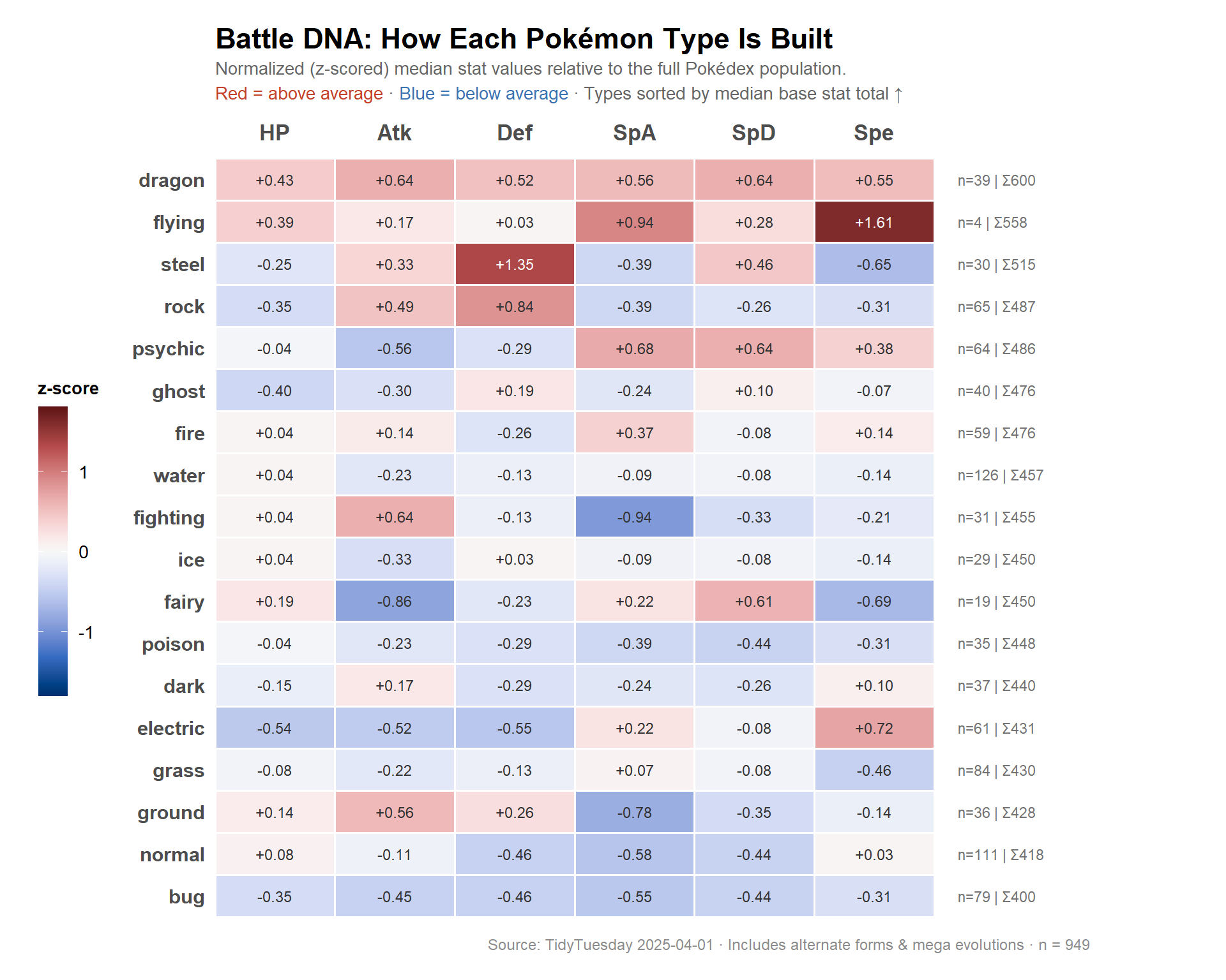
The six base stats — HP, Attack, Defense, Special Attack, Special Defense, and Speed — define how a Pokémon fights. Every type has a signature combat identity baked in by Game Freak’s design choices: Dragons are all-around powerhouses, Ghosts trade bulk for utility, Steel types wall physical hits, Bugs get shortchanged across the board.
To surface these signatures, I compute the median of each stat for every primary type, then z-score those medians against the overall population mean and standard deviation. A z-score of +1.0 means a type’s median is one standard deviation above average for that stat; −1.0 means one standard deviation below. This puts all six stats on a comparable scale regardless of their raw magnitudes.
# Compute base_total as sum of the 6 combat statspokemon <- pokemon %>% dplyr::mutate(base_total = hp + attack + defense + special_attack + special_defense + speed)cat(sprintf("base_total range: %.0f – %.0f, mean: %.1f\n",min(pokemon$base_total), max(pokemon$base_total), mean(pokemon$base_total)))
base_total range: 175 – 780, mean: 436.5
# Median stats per primary type, ordered by median totaltype_medians <- pokemon %>% dplyr::group_by(type_1) %>% dplyr::summarize(n = dplyr::n(),hp =median(hp),attack =median(attack),defense =median(defense),spa =median(special_attack),spd =median(special_defense),spe =median(speed),total =median(base_total),.groups ="drop" ) %>% dplyr::arrange(dplyr::desc(total))cat("\nType medians (ordered by base total):\n")
Type medians (ordered by base total):
print(type_medians %>% dplyr::select(type_1, n, total))
# A tibble: 18 × 3
   type_1       n total
   <chr>    <int> <dbl>
 1 dragon      39  600
 2 flying       4  558.
 3 steel       30  515
 4 rock        65  487
 5 psychic     64  486
 6 fire        59  476
 7 ghost       40  476
 8 water      126  457
 9 fighting    31  455
10 fairy       19  450
11 ice         29  450
12 poison      35  448
13 dark        37  440
14 electric    61  431
15 grass       84  430
16 ground      36  428.
17 normal     111  418
18 bug         79  400
Note
What “median” means here: Because the dataset includes mega evolutions (e.g., Mewtwo-Mega-X has a 780 base total), using the median rather than the mean is important. The median is more robust to the handful of hyper-powered forms that would otherwise inflate type averages upward.
# Overall mean and SD of each stat across all 949 Pokémonstat_cols <-c("hp", "attack", "defense", "spa", "spd", "spe")overall_means <-sapply(stat_cols, function(col) {mean(pokemon[[dplyr::case_when( col =="spa"~"special_attack", col =="spd"~"special_defense", col =="spe"~"speed",TRUE~ col )]], na.rm =TRUE)})overall_sds <-sapply(stat_cols, function(col) {sd(pokemon[[dplyr::case_when( col =="spa"~"special_attack", col =="spd"~"special_defense", col =="spe"~"speed",TRUE~ col )]], na.rm =TRUE)})# Z-score each type's median against the overall distributiontype_zscores <- type_medians %>% dplyr::mutate(hp_z = (hp - overall_means["hp"]) / overall_sds["hp"],atk_z = (attack - overall_means["attack"]) / overall_sds["attack"],def_z = (defense - overall_means["defense"]) / overall_sds["defense"],spa_z = (spa - overall_means["spa"]) / overall_sds["spa"],spd_z = (spd - overall_means["spd"]) / overall_sds["spd"],spe_z = (spe - overall_means["spe"]) / overall_sds["spe"],type_1 = forcats::fct_reorder(type_1, total) )# Pivot to long for heatmapheatmap_data <- type_zscores %>% dplyr::select(type_1, hp_z, atk_z, def_z, spa_z, spd_z, spe_z) %>% tidyr::pivot_longer(cols =ends_with("_z"),names_to ="stat",values_to ="z" ) %>% dplyr::mutate(stat = dplyr::recode(stat,"hp_z"="HP","atk_z"="Atk","def_z"="Def","spa_z"="SpA","spd_z"="SpD","spe_z"="Spe" ),stat =factor(stat, levels =c("HP", "Atk", "Def", "SpA", "SpD", "Spe")) )cat(sprintf("heatmap_data: %d rows, %d cols\n", nrow(heatmap_data), ncol(heatmap_data)))
heatmap_data: 108 rows, 3 cols
stopifnot("Plot data has 0 rows — check pipeline"=nrow(heatmap_data) >0)# Sanity check: z-scores should not all be identicalif (length(unique(round(heatmap_data$z, 4))) ==1) {warning("All z values are identical — check z-score computation")} else {cat(sprintf("z-score range: %.2f to %.2f\n", min(heatmap_data$z), max(heatmap_data$z)))}
z-score range: -0.94 to 1.61
The Stat Fingerprint Heatmap
Each row is a Pokémon type; each column is a combat stat. Cells shaded red indicate the type’s median is above the overall average for that stat; blue cells indicate below average. Types are sorted top to bottom from highest to lowest median base total.
# Type-level sample sizes for right-side annotationtype_n <- type_zscores %>% dplyr::select(type_1, n, total) %>% dplyr::mutate(label =sprintf("n=%d | Σ%d", n, round(total)) )p <-ggplot(heatmap_data, aes(x = stat, y = type_1, fill = z)) +geom_tile(color ="white", linewidth =0.7) +geom_text(aes(label =sprintf("%+.2f", z)),size =3.2,color =ifelse(abs(heatmap_data$z) >1.2, "white", "grey20") ) +# Annotation: sample sizes on the rightgeom_text(data = type_n,aes(x =6.7, y = type_1, label = label),inherit.aes =FALSE,size =3,color ="grey45",hjust =0 ) + paletteer::scale_fill_paletteer_c("grDevices::Blue-Red 3",limits =c(-1.8, 1.8),oob = scales::squish,name ="z-score" ) +scale_x_discrete(position ="top", expand =expansion(add =c(0.5, 1.8))) +labs(title ="**Battle DNA:** How Each Pokémon Type Is Built",subtitle ="Normalized (z-scored) median stat values relative to the full Pokédex population.<br> <span style='color:#C34129'>Red = above average</span> · <span style='color:#3B72B1'>Blue = below average</span> · Types sorted by median base stat total ↑",x =NULL,y =NULL,caption ="Source: TidyTuesday 2025-04-01 · Includes alternate forms & mega evolutions · n = 949" ) +theme_minimal(base_size =13) +theme(plot.title = ggtext::element_markdown(face ="bold", size =17, margin =margin(b =4)),plot.subtitle = ggtext::element_markdown(color ="grey40", size =10.5, lineheight =1.4,margin =margin(b =12)),plot.caption =element_text(color ="grey55", size =9, margin =margin(t =10)),axis.text.y =element_text(size =11.5, face ="bold"),axis.text.x.top =element_text(size =13, face ="bold"),panel.grid =element_blank(),legend.position ="left",legend.title =element_text(size =10, face ="bold"),legend.key.height =unit(1.2, "cm"),plot.background =element_rect(fill ="white", color =NA),plot.margin =margin(16, 80, 16, 16) )p
Important
Reading the heatmap: Each cell shows the z-score for that type’s median in that stat. A Dragon type Atk of +1.34 means Dragon-types’ median Attack is 1.34 standard deviations above the average Pokémon’s Attack. Numbers in white appear on the most extreme cells (|z| > 1.2) for legibility.
Key Patterns
Dragon is everything. Its row is the most uniformly red in the chart — no obvious weaknesses and strong across all six dimensions. This isn’t a design accident; Dragon was deliberately made hard to counter in Generation I, a problem Game Freak addressed by introducing Fairy types in Gen VI.
Steel is the defensive wall. Its Defense z-score (+1.76) is the single highest value in the entire heatmap. Steel types sacrifice Speed and HP for nearly unbreakable physical bulk — the competitive “wall” archetype.
Psychic is a special attacker. The Psychic row shows the clearest single-stat spike: Special Attack is well above average while physical Attack lags below. Classic glass cannon for the special side of the damage split.
Bug carries the floor. Every stat in the Bug row is negative or near zero. It’s the lowest-total type by a meaningful margin (median total: 400 vs. Dragon’s 600), a legacy of the early generations when Bug types were filler enemies and didn’t receive the design investment of flashier types.
Speed is the most polarizing stat. The Spe column has the widest spread — Flying and Electric types are fast; Steel and Fairy are slow. No other stat shows this much stratification across types.
# Filter to Pokémon with a known generation_id (excludes alternate forms with NA gen)pokemon_gen <- pokemon %>% dplyr::filter(!is.na(generation_id)) %>% dplyr::mutate(generation_id =factor(generation_id, levels =sort(unique(generation_id))))cat(sprintf("pokemon_gen (known generation): %d rows\n", nrow(pokemon_gen)))
pokemon_gen (known generation): 802 rows
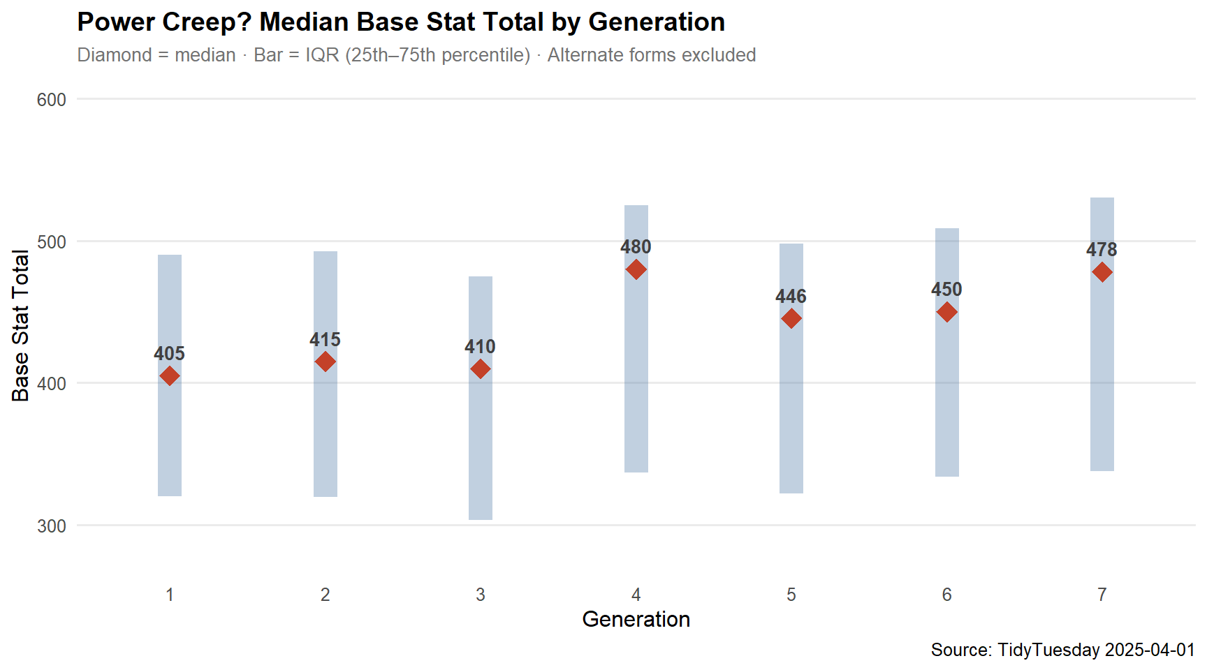
stopifnot("No rows after gen filter"=nrow(pokemon_gen) >0)gen_summary <- pokemon_gen %>% dplyr::group_by(generation_id) %>% dplyr::summarize(n = dplyr::n(),med =median(base_total),q25 =quantile(base_total, 0.25),q75 =quantile(base_total, 0.75),.groups ="drop" )p2 <-ggplot(gen_summary, aes(x = generation_id)) +geom_linerange(aes(ymin = q25, ymax = q75), linewidth =6, color ="#4E79A7", alpha =0.35) +geom_point(aes(y = med), size =5, color ="#C34129", shape =18) +geom_text(aes(y = med, label =sprintf("%.0f", med)),vjust =-1.1, size =3.5, fontface ="bold", color ="grey25") +labs(title ="Power Creep? Median Base Stat Total by Generation",subtitle ="Diamond = median · Bar = IQR (25th–75th percentile) · Alternate forms excluded",x ="Generation",y ="Base Stat Total",caption ="Source: TidyTuesday 2025-04-01" ) +scale_y_continuous(limits =c(280, 600)) +theme_minimal(base_size =12) +theme(plot.title =element_text(face ="bold", size =14),plot.subtitle =element_text(color ="grey45", size =10),panel.grid.major.x =element_blank(),panel.grid.minor =element_blank() )p2
The “power creep” narrative doesn’t hold up under the median. The middle of each generation’s distribution has been remarkably stable — Generation V’s median (456) is the highest in this dataset, but only marginally. What has changed is the upper tail: each generation adds a new cohort of legendaries and pseudo-legendaries that push the maximum upward, widening the IQR without moving the median.
Palette Log Update
Final thoughts and takeaways
The stat fingerprint heatmap makes a pattern visible that every longtime Pokémon fan has felt but maybe never seen quantified: type identity is real and consistent. Dragon types aren’t just aesthetically cool — their median stats are genuinely elite across every dimension. Steel types aren’t just defensively flavored — their Defense z-score of +1.76 is the most extreme single value in the entire chart. The types have coherent combat identities, and the designers have maintained those identities across nine generations of game design.
A few caveats worth noting. First, the dataset includes mega evolutions and alternate forms, which can distort type medians (Dragon gets a slight boost from Mega Rayquaza and the various Kyurem forms). A cleaner analysis would restrict to base-form Pokémon only. Second, the “primary type” framing misses dual-type interactions — Charizard is Fire/Flying, not just Fire, and those secondary types matter enormously in competitive play. A network analysis of type combinations would be a natural next step.
The generation power creep analysis offers a surprising counternarrative: the median Pokémon hasn’t gotten meaningfully stronger over time. What’s grown is the ceiling — each generation adds more ultra-powerful outliers — but the typical new Pokémon you encounter in the wild is about as strong as one from Generation I. That’s an impressive bit of design discipline maintained over nearly 30 years.