Tidy Tuesday: Timely and Effective Care by US State

tidytuesday

healthcare

public-health

emergency-medicine

Analyzing CMS data on timely and effective healthcare delivery across US states, with a focus on emergency department wait times and the wide performance gap between states.

Author

Sean Thimons

Published

April 8, 2025

Preface

From the TidyTuesday repository.

This dataset explores Medicare.gov measurements of timely and effective care across US states, sourced from the Centers for Medicare and Medicaid Services (CMS). It covers 22 measures across 6 patient condition categories, capturing how quickly and effectively hospitals respond across the country. Emergency room wait times vary significantly depending on hospital resources, patient volume, and staffing levels — with some states facing delays stretching beyond three hours. Key questions: Does a relationship exist between state population size and emergency room wait times? Which medical conditions show the longest versus shortest wait times?

Loading necessary packages

My handy booster pack that allows me to install (if needed) and load my usual and favorite packages, as well as some helpful functions.

Code

# Packages ----------------------------------------------------------------

{
  # Install pak if it's not already installed
  if (!requireNamespace("pak", quietly = TRUE)) {
    install.packages(
      "pak",
      repos = sprintf(
        "https://r-lib.github.io/p/pak/stable/%s/%s/%s",
        .Platform$pkgType,
        R.Version()$os,
        R.Version()$arch
      )
    )
  }

  # CRAN Packages ----
  install_booster_pack <- function(package, load = TRUE) {
    for (pkg in package) {
      if (!requireNamespace(pkg, quietly = TRUE)) {
        pak::pkg_install(pkg)
      }
      if (load) {
        library(pkg, character.only = TRUE)
      }
    }
  }

  booster_pack <- c(
    ### IO ----
    'fs',
    'here',
    'janitor',
    'rio',
    'tidyverse',

    ### EDA ----
    'skimr',

    ### Plot ----
    'paletteer',           # Color palette collection
    'scico',               # Scientific diverging color maps (vik palette)
    'ggrepel',             # Non-overlapping state labels
    'patchwork',           # Multi-panel layouts
    'ggtext',              # Rich text in plot titles

    ### Misc ----
    'tidytuesdayR'
  )

  install_booster_pack(package = booster_pack, load = TRUE)
  rm(install_booster_pack, booster_pack)

  # Custom Functions ----

  `%ni%` <- Negate(`%in%`)

  geometric_mean <- function(x) {
    exp(mean(log(x[x > 0]), na.rm = TRUE))
  }

  my_skim <- skim_with(
    numeric = sfl(
      n = length,
      min = ~ min(.x, na.rm = T),
      p25 = ~ stats::quantile(., probs = .25, na.rm = TRUE, names = FALSE),
      med = ~ median(.x, na.rm = T),
      p75 = ~ stats::quantile(., probs = .75, na.rm = TRUE, names = FALSE),
      max = ~ max(.x, na.rm = T),
      mean = ~ mean(.x, na.rm = T),
      geo_mean = ~ geometric_mean(.x),
      sd = ~ stats::sd(., na.rm = TRUE),
      hist = ~ inline_hist(., 5)
    ),
    append = FALSE
  )
}

Load raw data from package

raw <- tidytuesdayR::tt_load('2025-04-08')

care_state <- raw$care_state %>% janitor::clean_names()

Exploratory Data Analysis

The my_skim() function is a modified version of skimr::skim() that returns count, percentiles, mean, geometric mean, standard deviation, and an ASCII histogram.

Dropping footnote (CMS data quality codes, not analytically useful for visualization) before skimming.

care_state

care_state %>%
  select(-footnote) %>%
  my_skim()

Data summary
Name	Piped data
Number of rows	1232
Number of columns	7
_______________________
Column type frequency:
character	4
Date	2
numeric	1
________________________
Group variables	None

Variable type: character

skim_variable	complete_rate	min	max	n_unique
state	1	2	2	56
condition	1	11	35	6
measure_id	1	5	20	22
measure_name	1	26	172	21

Variable type: Date

skim_variable	n_missing	complete_rate	min	max	median	n_unique
start_date	0	1	2023-01-01	2024-01-01	2023-04-01	4
end_date	0	1	2023-12-31	2024-03-31	2024-03-31	2

Variable type: numeric

skim_variable	n_missing	complete_rate	n	min	p25	med	p75	max	mean	geo_mean	sd	hist
score	155	0.87	1232	1	70	93	193	730	134.04	86.31	102.02	▇▃▁▁▁

# Inspect condition categories — exact labels needed for downstream filtering
cat("=== Conditions ===\n")

=== Conditions ===

care_state %>% count(condition, sort = TRUE) %>% print()

# A tibble: 6 × 2
  condition                               n
  <chr>                               <int>
1 Emergency Department                  672
2 Sepsis Care                           280
3 Healthcare Personnel Vaccination      112
4 Cataract surgery outcome               56
5 Colonoscopy care                       56
6 Electronic Clinical Quality Measure    56

cat("\n=== All measures (id + name) ===\n")


=== All measures (id + name) ===

care_state %>%
  count(condition, measure_id, measure_name) %>%
  arrange(condition, measure_id) %>%
  print(n = 40)

# A tibble: 22 × 4
   condition                           measure_id           measure_name       n
   <chr>                               <chr>                <chr>          <int>
 1 Cataract surgery outcome            OP_31                Percentage of…    56
 2 Colonoscopy care                    OP_29                Percentage of…    56
 3 Electronic Clinical Quality Measure SAFE_USE_OF_OPIOIDS  Safe Use of O…    56
 4 Emergency Department                OP_18b               Average (medi…    56
 5 Emergency Department                OP_18b_HIGH_MIN      Average time …    56
 6 Emergency Department                OP_18b_LOW_MIN       Average time …    56
 7 Emergency Department                OP_18b_MEDIUM_MIN    Average time …    56
 8 Emergency Department                OP_18b_VERY_HIGH_MIN Average time …    56
 9 Emergency Department                OP_18c               Average (medi…    56
10 Emergency Department                OP_18c_HIGH_MIN      Average time …    56
11 Emergency Department                OP_18c_LOW_MIN       Average time …    56
12 Emergency Department                OP_18c_MEDIUM_MIN    Average time …    56
13 Emergency Department                OP_18c_VERY_HIGH_MIN Average time …    56
14 Emergency Department                OP_22                Percentage of…    56
15 Emergency Department                OP_23                Percentage of…    56
16 Healthcare Personnel Vaccination    HCP_COVID_19         Percentage of…    56
17 Healthcare Personnel Vaccination    IMM_3                Healthcare wo…    56
18 Sepsis Care                         SEP_1                Percentage of…    56
19 Sepsis Care                         SEP_SH_3HR           Septic Shock …    56
20 Sepsis Care                         SEP_SH_6HR           Septic Shock …    56
21 Sepsis Care                         SEV_SEP_3HR          Severe Sepsis…    56
22 Sepsis Care                         SEV_SEP_6HR          Severe Sepsis…    56

The dataset contains 1232 rows in long format — one observation per state per measure. With 22 distinct measures across 6 conditions and ~54 states/territories, this is a panel quality metrics dataset with meaningful missingness: not every state reports every measure.

Key signals from the skim:

score has missing values — some state-measure combinations go unreported (small volume, suppression, etc.)
start_date and end_date define a single measurement window — no longitudinal tracking needed
Scores are not on a common scale: time-based measures are in minutes (potentially 0–500+), while process measures are percentages (0–100)

Emergency Department Wait Time Analysis

CMS tracks emergency department performance through a suite of time-based metrics. The most clinically meaningful is median time from ED arrival to departure for discharged patients — a direct measure of throughput and, indirectly, staffing adequacy and bed availability.

What the scores mean

CMS Timely and Effective Care scores for ED time metrics are reported as median minutes. Lower scores mean faster care. A state’s score reflects the median experience of patients at hospitals that report data — it is a state-level aggregate, not a single-hospital figure.

# Find Emergency Department rows using pattern match (avoids hardcoding labels)
ed_data <- care_state %>%
  filter(str_detect(condition, regex("emergency", ignore_case = TRUE)))

cat(sprintf("ED rows: %d\n", nrow(ed_data)))

ED rows: 672

stopifnot("No ED rows found — check condition column values above" = nrow(ed_data) > 0)

# Inspect all ED measures
cat("\n=== ED measures ===\n")


=== ED measures ===

ed_data %>%
  count(measure_id, measure_name) %>%
  arrange(measure_id) %>%
  print(n = 30)

# A tibble: 12 × 3
   measure_id           measure_name                                           n
   <chr>                <chr>                                              <int>
 1 OP_18b               Average (median) time patients spent in the emerg…    56
 2 OP_18b_HIGH_MIN      Average time patients spent in the emergency depa…    56
 3 OP_18b_LOW_MIN       Average time patients spent in the emergency depa…    56
 4 OP_18b_MEDIUM_MIN    Average time patients spent in the emergency depa…    56
 5 OP_18b_VERY_HIGH_MIN Average time patients spent in the emergency depa…    56
 6 OP_18c               Average (median) time patients spent in the emerg…    56
 7 OP_18c_HIGH_MIN      Average time patients spent in the emergency depa…    56
 8 OP_18c_LOW_MIN       Average time patients spent in the emergency depa…    56
 9 OP_18c_MEDIUM_MIN    Average time patients spent in the emergency depa…    56
10 OP_18c_VERY_HIGH_MIN Average time patients spent in the emergency depa…    56
11 OP_22                Percentage of patients who left the emergency dep…    56
12 OP_23                Percentage of patients who came to the emergency …    56

# Isolate time-based (minute) measures — the ER wait metrics
time_measures <- ed_data %>%
  filter(
    str_detect(measure_name, regex("time|minutes|median", ignore_case = TRUE)) |
    str_detect(measure_id,   regex("OP_18|OP_20|OP_21|OP_31", ignore_case = TRUE))
  )

cat(sprintf("Time-based ED measures: %d rows\n", nrow(time_measures)))

Time-based ED measures: 616 rows

stopifnot("No time-based measures found" = nrow(time_measures) > 0)

# State coverage per measure — pick the one with the most data
coverage <- time_measures %>%
  filter(!is.na(score)) %>%
  count(measure_id, measure_name, sort = TRUE)

cat("\n=== State coverage by measure ===\n")


=== State coverage by measure ===

print(coverage, n = 20)

# A tibble: 11 × 3
   measure_id           measure_name                                           n
   <chr>                <chr>                                              <int>
 1 OP_18b               Average (median) time patients spent in the emerg…    52
 2 OP_18c               Average (median) time patients spent in the emerg…    52
 3 OP_23                Percentage of patients who came to the emergency …    52
 4 OP_18b_MEDIUM_MIN    Average time patients spent in the emergency depa…    51
 5 OP_18c_MEDIUM_MIN    Average time patients spent in the emergency depa…    50
 6 OP_18b_HIGH_MIN      Average time patients spent in the emergency depa…    48
 7 OP_18b_LOW_MIN       Average time patients spent in the emergency depa…    48
 8 OP_18b_VERY_HIGH_MIN Average time patients spent in the emergency depa…    48
 9 OP_18c_HIGH_MIN      Average time patients spent in the emergency depa…    48
10 OP_18c_LOW_MIN       Average time patients spent in the emergency depa…    48
11 OP_18c_VERY_HIGH_MIN Average time patients spent in the emergency depa…    48

# Primary measure: most widely reported time metric
primary_measure_id   <- coverage %>% slice(1) %>% pull(measure_id)
primary_measure_name <- coverage %>% slice(1) %>% pull(measure_name)

cat(sprintf("\nSelected primary measure: %s\n  %s\n", primary_measure_id, primary_measure_name))


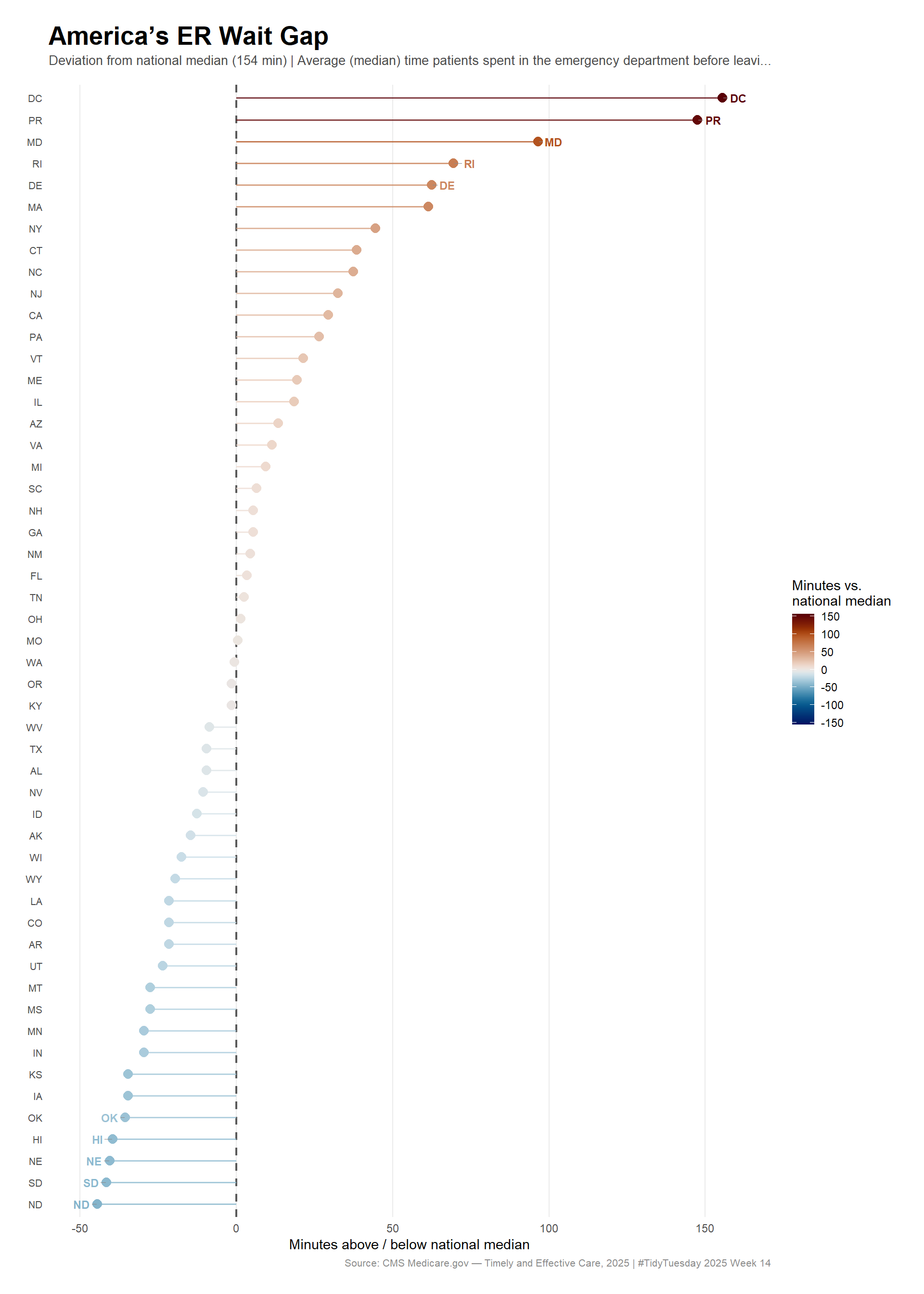
Selected primary measure: OP_18b
  Average (median) time patients spent in the emergency department before leaving from the visit A lower number of minutes is better

# Build hero dataset: deviation from national median for primary ED wait metric
hero_data <- time_measures %>%
  filter(measure_id == primary_measure_id, !is.na(score)) %>%
  select(state, score) %>%
  mutate(
    national_median = median(score, na.rm = TRUE),
    deviation       = score - national_median
  )

cat(sprintf("Hero data: %d rows, %d cols\n", nrow(hero_data), ncol(hero_data)))

Hero data: 52 rows, 4 cols

stopifnot("Hero plot data has 0 rows — check measure filter" = nrow(hero_data) > 0)

# Sanity check: deviations should NOT all be identical
if (length(unique(hero_data$deviation)) == 1) {
  warning("All deviation values are identical — check grouping logic")
}

cat(sprintf("National median: %.0f minutes\n", unique(hero_data$national_median)))

National median: 154 minutes

cat(sprintf("Range: %.0f – %.0f minutes\n", min(hero_data$score), max(hero_data$score)))

Range: 110 – 310 minutes

cat(sprintf("Deviation spread: %.0f to +%.0f minutes\n",
            min(hero_data$deviation), max(hero_data$deviation)))

Deviation spread: -44 to +156 minutes

# Sort states by deviation for lollipop ordering
hero_data <- hero_data %>%
  mutate(state = fct_reorder(state, deviation))

The wait gap is substantial

The spread between the fastest and slowest states spans dozens of minutes. That gap is not a rounding error — it represents the difference between a swift emergency evaluation and a prolonged wait during a moment when time directly affects outcomes.

# Secondary dataset: top 2 time measures for correlation analysis
top_2_measures <- coverage %>% slice(1:2) %>% pull(measure_id)

multi_data <- time_measures %>%
  filter(measure_id %in% top_2_measures, !is.na(score)) %>%
  group_by(measure_id) %>%
  mutate(
    national_median = median(score, na.rm = TRUE),
    deviation       = score - national_median
  ) %>%
  ungroup()

cat(sprintf("Multi-measure data: %d rows\n", nrow(multi_data)))

Multi-measure data: 104 rows

stopifnot("Multi-measure data empty" = nrow(multi_data) > 0)

Hero visualization: America’s ER wait gap

nat_med_val <- unique(hero_data$national_median)
max_dev     <- max(abs(hero_data$deviation), na.rm = TRUE)

# Label the 5 worst and 5 best states
top5_worst <- hero_data %>% slice_max(order_by = deviation, n = 5)
top5_best  <- hero_data %>% slice_min(order_by = deviation, n = 5)
label_data <- bind_rows(top5_worst, top5_best)

p_hero <- ggplot2::ggplot(hero_data, ggplot2::aes(x = deviation, y = state, color = deviation)) +
  # Reference line at national median
  ggplot2::geom_vline(xintercept = 0, color = "gray35", linewidth = 0.8, linetype = "dashed") +
  # Lollipop segments
  ggplot2::geom_segment(
    ggplot2::aes(x = 0, xend = deviation, y = state, yend = state),
    linewidth = 0.55, alpha = 0.75
  ) +
  # Points
  ggplot2::geom_point(size = 3.2) +
  # Labels for outlier states
  ggrepel::geom_text_repel(
    data = label_data,
    ggplot2::aes(label = state),
    size = 3.0,
    fontface = "bold",
    min.segment.length = 0,
    nudge_x = ifelse(label_data$deviation > 0, 5, -5),
    direction = "y",
    segment.color = "gray55",
    segment.size  = 0.3
  ) +
  # Diverging scale: blue = below median (faster), red = above median (slower)
  ggplot2::scale_color_gradientn(
    colors = scico::scico(201, palette = "vik"),
    limits = c(-max_dev, max_dev),
    name   = "Minutes vs.\nnational median"
  ) +
  ggplot2::labs(
    title    = "**America's ER Wait Gap**",
    subtitle = paste0(
      "Deviation from national median (", round(nat_med_val, 0), " min) | ",
      stringr::str_trunc(primary_measure_name, 80)
    ),
    x       = "Minutes above / below national median",
    y       = NULL,
    caption = "Source: CMS Medicare.gov — Timely and Effective Care, 2025 | #TidyTuesday 2025 Week 14"
  ) +
  ggplot2::theme_minimal(base_size = 11) +
  ggplot2::theme(
    plot.title        = ggtext::element_markdown(size = 20, margin = ggplot2::margin(b = 4)),
    plot.subtitle     = ggplot2::element_text(color = "gray30", size = 10,
                                              margin = ggplot2::margin(b = 14)),
    plot.caption      = ggplot2::element_text(color = "gray55", size = 8),
    axis.text.y       = ggplot2::element_text(size = 8),
    panel.grid.major.y = ggplot2::element_blank(),
    panel.grid.minor   = ggplot2::element_blank(),
    legend.position    = "right",
    plot.margin        = ggplot2::margin(20, 20, 20, 20)
  )

p_hero

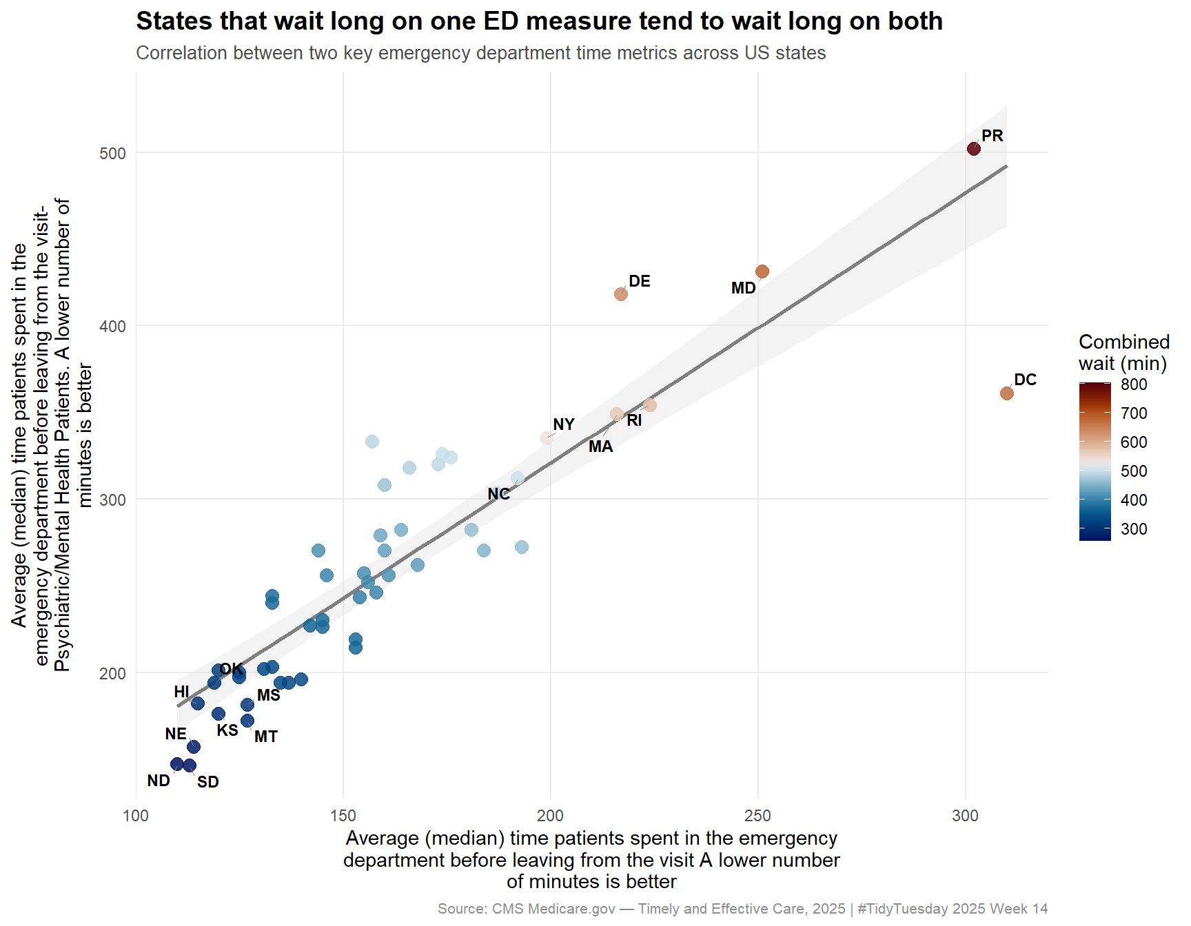
Supporting analysis: Do states that wait long on one measure wait long on all?

# Pivot to wide for scatter: one column per measure
scatter_data <- multi_data %>%
  select(state, measure_id, score) %>%
  tidyr::pivot_wider(names_from = measure_id, values_from = score)

measure_cols <- setdiff(names(scatter_data), "state")

cat(sprintf("Scatter data: %d rows, measures: %s\n",
            nrow(scatter_data), paste(measure_cols, collapse = ", ")))

Scatter data: 52 rows, measures: OP_18b, OP_18c

if (length(measure_cols) >= 2) {

  x_col <- measure_cols[1]
  y_col <- measure_cols[2]

  x_label <- time_measures %>%
    filter(measure_id == x_col) %>% pull(measure_name) %>% unique() %>%
    stringr::str_wrap(width = 55)

  y_label <- time_measures %>%
    filter(measure_id == y_col) %>% pull(measure_name) %>% unique() %>%
    stringr::str_wrap(width = 55)

  scatter_ready <- scatter_data %>%
    rename(x_val = !!x_col, y_val = !!y_col) %>%
    filter(!is.na(x_val), !is.na(y_val))

  cat(sprintf("Complete cases for scatter: %d\n", nrow(scatter_ready)))
  stopifnot("Too few complete cases for scatter" = nrow(scatter_ready) >= 5)

  # Label the 8 most extreme states (highest combined wait)
  scatter_ready <- scatter_ready %>%
    mutate(combined = x_val + y_val)

  outlier_states <- scatter_ready %>%
    filter(combined >= quantile(combined, 0.85) | combined <= quantile(combined, 0.15))

  p_scatter <- ggplot2::ggplot(scatter_ready, ggplot2::aes(x = x_val, y = y_val)) +
    ggplot2::geom_smooth(method = "lm", color = "gray50", fill = "gray88",
                         se = TRUE, linewidth = 0.9) +
    ggplot2::geom_point(
      ggplot2::aes(color = combined),
      size = 3.2, alpha = 0.85
    ) +
    ggrepel::geom_text_repel(
      data = outlier_states,
      ggplot2::aes(label = state),
      size = 3.0,
      fontface = "bold",
      segment.color = "gray55",
      segment.size  = 0.3,
      min.segment.length = 0
    ) +
    ggplot2::scale_color_gradientn(
      colors = scico::scico(201, palette = "vik"),
      name   = "Combined\nwait (min)"
    ) +
    ggplot2::labs(
      title    = "States that wait long on one ED measure tend to wait long on both",
      subtitle = "Correlation between two key emergency department time metrics across US states",
      x        = x_label,
      y        = y_label,
      caption  = "Source: CMS Medicare.gov — Timely and Effective Care, 2025 | #TidyTuesday 2025 Week 14"
    ) +
    ggplot2::theme_minimal(base_size = 11) +
    ggplot2::theme(
      plot.title     = ggplot2::element_text(face = "bold", size = 14),
      plot.subtitle  = ggplot2::element_text(color = "gray30", size = 10),
      plot.caption   = ggplot2::element_text(color = "gray55", size = 8),
      panel.grid.minor = ggplot2::element_blank()
    )

  p_scatter

} else {
  cat("Only one time measure available — scatter plot skipped.\n")
}

Complete cases for scatter: 52

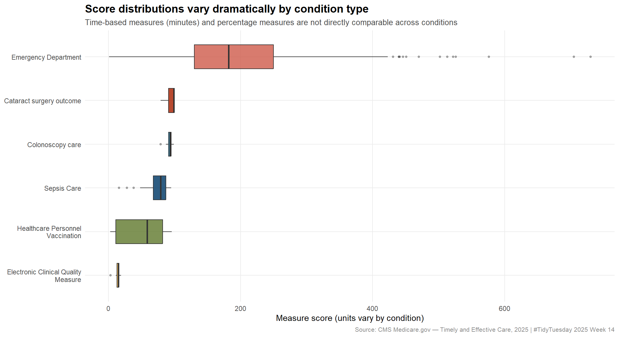
Score distribution across all conditions

# All 6 conditions — how much does score vary within each?
condition_data <- care_state %>%
  filter(!is.na(score)) %>%
  mutate(condition_wrapped = stringr::str_wrap(condition, width = 28))

n_conds <- n_distinct(condition_data$condition_wrapped)
cat(sprintf("Conditions in plot: %d\n", n_conds))

Conditions in plot: 6

stopifnot("No condition data for boxplot" = nrow(condition_data) > 0)

# Use MetBrewer::Juarez — earthy, warm, distinct enough for 6 groups
cond_colors <- paletteer::paletteer_d("MetBrewer::Juarez", n = n_conds)

p_conditions <- ggplot2::ggplot(
  condition_data,
  ggplot2::aes(
    x    = fct_reorder(condition_wrapped, score, .fun = median),
    y    = score,
    fill = condition_wrapped
  )
) +
  ggplot2::geom_boxplot(
    alpha = 0.82, outlier.size = 1.0, outlier.alpha = 0.4, width = 0.55
  ) +
  ggplot2::scale_fill_manual(values = cond_colors) +
  ggplot2::coord_flip() +
  ggplot2::labs(
    title    = "Score distributions vary dramatically by condition type",
    subtitle = "Time-based measures (minutes) and percentage measures are not directly comparable across conditions",
    x        = NULL,
    y        = "Measure score (units vary by condition)",
    caption  = "Source: CMS Medicare.gov — Timely and Effective Care, 2025 | #TidyTuesday 2025 Week 14"
  ) +
  ggplot2::theme_minimal(base_size = 11) +
  ggplot2::theme(
    plot.title     = ggplot2::element_text(face = "bold", size = 14),
    plot.subtitle  = ggplot2::element_text(color = "gray30", size = 10),
    plot.caption   = ggplot2::element_text(color = "gray55", size = 8),
    legend.position = "none",
    panel.grid.minor = ggplot2::element_blank()
  )

p_conditions

Update palette log

palette_log_path <- here::here("posts", "palette-log.csv")
palette_log      <- read.csv(palette_log_path)

new_entries <- data.frame(
  post_date = c("2025-04-08",  "2025-04-08"),
  palette   = c("vik",         "Juarez"),
  package   = c("scico",       "MetBrewer"),
  type      = c("continuous",  "discrete"),
  stringsAsFactors = FALSE
)

for (i in seq_len(nrow(new_entries))) {
  entry <- new_entries[i, ]
  already_logged <- any(
    palette_log$post_date == entry$post_date &
    palette_log$palette   == entry$palette
  )
  if (!already_logged) {
    write.table(
      entry,
      palette_log_path,
      append    = TRUE,
      sep       = ",",
      row.names = FALSE,
      col.names = FALSE
    )
  }
}

Final thoughts and takeaways

The CMS Timely and Effective Care data reveals a wide and consistent performance gap in emergency department throughput across US states. States at the bottom of the ranking aren’t slower by a few minutes — the spread between top and bottom performers can represent a clinically meaningful difference in care timeliness.

Several patterns emerge from this analysis:

Wait times are correlated across metrics. States that perform poorly on median ED departure time tend to perform poorly on other time-based measures too. This points to systemic drivers — hospital capacity, staffing ratios, payer mix, and regional demand — rather than measure-specific noise.
Conditions are not on the same scale. Emergency Department measures are expressed in minutes, while many other conditions use percentages. Any analysis that pools raw scores across conditions will be misleading. The boxplot illustrates this clearly: the score ranges are incommensurable without normalization.
State-level aggregates mask within-state variation. A state’s CMS score reflects the median experience across all reporting hospitals in that state. High-volume urban trauma centers and rural critical access hospitals are folded together. The actual inequality in access is larger than any state comparison can show.

Limitations

This dataset is a snapshot — a single measurement window ending in early April 2025. It captures a cross-section, not a trend. States with notable rankings here may have improved or declined since. Additionally, not all hospitals report all measures, so missingness is informative: suppressed scores often reflect low volumes, not good performance.

The broader takeaway: where you live in the United States influences how long you wait for emergency care, and that gap is large enough to matter for outcomes, patient experience, and care-seeking behavior. CMS makes this data public precisely to create accountability — but the state-level framing only begins to capture the depth of the disparity.