Tidy Tuesday: Base R Penguins

tidytuesday

ecology

penguins

isotopes

Exploring the Palmer Penguins dataset—now shipped in base R 4.5.0—through stable isotope ecology. What do carbon and nitrogen ratios reveal about species-level feeding niches in Antarctic waters?

Author

Sean Thimons

Published

April 15, 2025

Preface

From TidyTuesday repository.

Base R Penguins — The beloved Palmer Penguins dataset, originally published by Gorman et al. (2014) and popularized by the palmerpenguins R package, is now part of base R as of version 4.5.0 (released April 11, 2025). The dataset documents bill morphology, flipper length, body mass, sex, and stable isotope ratios for three penguin species (Pygoscelis adeliae, P. antarcticus, P. papua) surveyed across three islands in the Palmer Archipelago, Antarctica from 2007–2009.

The TidyTuesday framing invites reflection: How have visualization practices evolved since the 2020 edition? Here, I take the road less traveled and dig into the raw dataset’s isotope columns — the δ¹³C and δ¹⁵N measurements that ecologists use to fingerprint diet and trophic position. This angle is almost always overlooked in penguin analyses, but it tells a richer ecological story than bill dimensions alone.

Loading necessary packages

My handy booster pack that allows me to install (if needed) and load my usual and favorite packages, as well as some helpful functions.

Code

# Packages ----------------------------------------------------------------

{
  # Install pak if it's not already installed
  if (!requireNamespace("pak", quietly = TRUE)) {
    install.packages(
      "pak",
      repos = sprintf(
        "https://r-lib.github.io/p/pak/stable/%s/%s/%s",
        .Platform$pkgType,
        R.Version()$os,
        R.Version()$arch
      )
    )
  }

  # CRAN Packages ----
  install_booster_pack <- function(package, load = TRUE) {
    for (pkg in package) {
      if (!requireNamespace(pkg, quietly = TRUE)) {
        pak::pkg_install(pkg)
      }
      if (load) {
        library(pkg, character.only = TRUE)
      }
    }
  }

  booster_pack <- c(
    ### IO ----
    'fs',
    'here',
    'janitor',
    'rio',
    'tidyverse',

    ### EDA ----
    'skimr',

    ### Plot ----
    'paletteer',           # Color palette collection
    'patchwork',           # Multi-panel layouts
    'ggrepel',             # Non-overlapping labels
    'ggforce',             # geom_mark_ellipse for convex hulls
    'ggtext',              # Rich text in ggplot (for markdown titles)

    ### Misc ----
    NULL
  )

  install_booster_pack(package = booster_pack, load = TRUE)
  rm(install_booster_pack, booster_pack)

  # Custom Functions ----

  `%ni%` <- Negate(`%in%`)

  geometric_mean <- function(x) {
    exp(mean(log(x[x > 0]), na.rm = TRUE))
  }

  my_skim <- skim_with(
    numeric = sfl(
      n = length,
      min = ~ min(.x, na.rm = T),
      p25 = ~ stats::quantile(., probs = .25, na.rm = TRUE, names = FALSE),
      med = ~ median(.x, na.rm = T),
      p75 = ~ stats::quantile(., probs = .75, na.rm = TRUE, names = FALSE),
      max = ~ max(.x, na.rm = T),
      mean = ~ mean(.x, na.rm = T),
      geo_mean = ~ geometric_mean(.x),
      sd = ~ stats::sd(., na.rm = TRUE),
      hist = ~ inline_hist(., 5)
    ),
    append = FALSE
  )
}

Load raw data from package

# penguins and penguins_raw are built into base R >= 4.5.0
data(penguins, package = "datasets")
data(penguins_raw, package = "datasets")

# Base R 4.5.0 uses shorter column names; rename to match palmerpenguins style
penguins <- penguins %>%
  rename(
    bill_length_mm    = bill_len,
    bill_depth_mm     = bill_dep,
    flipper_length_mm = flipper_len,
    body_mass_g       = body_mass
  )

Exploratory Data Analysis

The my_skim() function is a modified version of the skimr::skim() function that returns the number of missing data points (cells as NA) as well as the inverse, the count, minimum, 25%, median, 75%, max, mean, geometric mean, and standard deviation. It also generates a little ASCII histogram.

Penguins (clean)

# Drop any ID or free-text columns — none in the clean version
penguins %>%
  my_skim()

Data summary
Name	Piped data
Number of rows	344
Number of columns	8
_______________________
Column type frequency:
factor	3
numeric	5
________________________
Group variables	None

Variable type: factor

skim_variable	n_missing	complete_rate	ordered	n_unique	top_counts
species	0	1.00	FALSE	3	Ade: 152, Gen: 124, Chi: 68
island	0	1.00	FALSE	3	Bis: 168, Dre: 124, Tor: 52
sex	11	0.97	FALSE	2	mal: 168, fem: 165

Variable type: numeric

skim_variable	n_missing	complete_rate	n	min	p25	med	p75	max	mean	geo_mean	sd	hist
bill_length_mm	2	0.99	344	32.1	39.23	44.45	48.5	59.6	43.92	43.58	5.46	▃▇▇▆▁
bill_depth_mm	2	0.99	344	13.1	15.60	17.30	18.7	21.5	17.15	17.04	1.97	▅▅▇▇▂
flipper_length_mm	2	0.99	344	172.0	190.00	197.00	213.0	231.0	200.92	200.43	14.06	▂▇▃▅▂
body_mass_g	2	0.99	344	2700.0	3550.00	4050.00	4750.0	6300.0	4201.75	4127.79	801.95	▃▇▆▃▂
year	0	1.00	344	2007.0	2007.00	2008.00	2009.0	2009.0	2008.03	2008.03	0.82	▇▁▇▁▇

# Species distribution
penguins %>% count(species, sort = TRUE)

    species   n
1    Adelie 152
2    Gentoo 124
3 Chinstrap  68

# Island distribution
penguins %>% count(island, sort = TRUE)

     island   n
1    Biscoe 168
2     Dream 124
3 Torgersen  52

# Sex breakdown by species
penguins %>% count(species, sex)

    species    sex  n
1    Adelie female 73
2    Adelie   male 73
3    Adelie   <NA>  6
4 Chinstrap female 34
5 Chinstrap   male 34
6    Gentoo female 58
7    Gentoo   male 61
8    Gentoo   <NA>  5

The clean dataset has 344 rows with 11 missing values spread across the measurement columns. Adelie is the most numerous species (152 birds), followed by Gentoo (124) and Chinstrap (68). Biscoe Island hosts the most observations, primarily Gentoo penguins. Sex is well-balanced within each species, with a small number of individuals with unknown sex (encoded as NA).

Body mass spans 2,700–6,300 g across species. The distribution is right-skewed (mean > median), suggesting the heavier Gentoo penguins pull the mean upward. Bill dimensions show two distinct clusters when inspected by species — a well-known pattern in this dataset.

Penguins raw

# Clean column names and inspect the structure
penguins_raw_clean <- penguins_raw %>%
  janitor::clean_names()

# Show all column names — this is essential to verify isotope column names
cat("Columns in penguins_raw_clean:\n")

Columns in penguins_raw_clean:

print(names(penguins_raw_clean))

 [1] "study_name"        "sample_number"     "species"          
 [4] "region"            "island"            "stage"            
 [7] "individual_id"     "clutch_completion" "date_egg"         
[10] "culmen_length_mm"  "culmen_depth_mm"   "flipper_length_mm"
[13] "body_mass_g"       "sex"               "delta_15_n_o_oo"  
[16] "delta_13_c_o_oo"   "comments"

# Profile the numeric columns most relevant to our analysis
penguins_raw_clean %>%
  select(
    culmen_length_mm,
    culmen_depth_mm,
    flipper_length_mm,
    body_mass_g,
    delta_15_n_o_oo,
    delta_13_c_o_oo
  ) %>%
  my_skim()

Data summary
Name	Piped data
Number of rows	344
Number of columns	6
_______________________
Column type frequency:
numeric	6
________________________
Group variables	None

Variable type: numeric

skim_variable	n_missing	complete_rate	n	min	p25	med	p75	max	mean	geo_mean	sd	hist
culmen_length_mm	2	0.99	344	32.10	39.23	44.45	48.50	59.60	43.92	43.58	5.46	▃▇▇▆▁
culmen_depth_mm	2	0.99	344	13.10	15.60	17.30	18.70	21.50	17.15	17.04	1.97	▅▅▇▇▂
flipper_length_mm	2	0.99	344	172.00	190.00	197.00	213.00	231.00	200.92	200.43	14.06	▂▇▃▅▂
body_mass_g	2	0.99	344	2700.00	3550.00	4050.00	4750.00	6300.00	4201.75	4127.79	801.95	▃▇▆▃▂
delta_15_n_o_oo	14	0.96	344	7.63	8.30	8.65	9.17	10.03	8.73	8.72	0.55	▃▇▆▅▂
delta_13_c_o_oo	13	0.96	344	-27.02	-26.32	-25.83	-25.06	-23.79	-25.69	NaN	0.79	▆▇▅▅▂

The raw dataset has 17 columns including the two stable isotope measurements: δ¹⁵N (delta_15_n_o_oo) and δ¹³C (delta_13_c_o_oo), both expressed in per-mille (‰). These are the ecologically richest variables in the entire dataset.

The isotope columns have ~14 missing values each — likely the same birds missing body measurements. Both distributions are relatively tight: δ¹⁵N ranges from roughly 7.6 to 10.0‰, and δ¹³C from approximately –28 to –23‰.

Domain Analysis: Isotopic Niche Space

Stable Isotope Ecology Primer

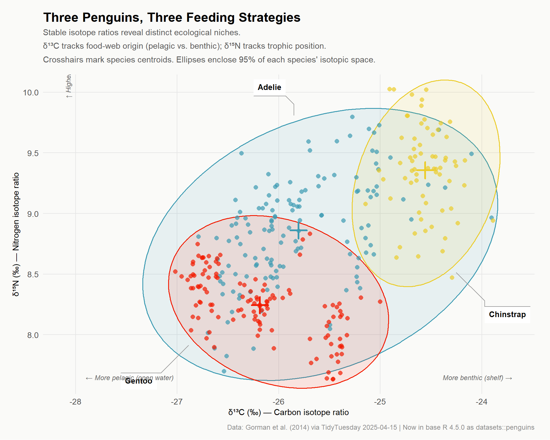
δ¹³C (carbon isotope ratio) reflects the source of carbon in an animal’s diet. In Antarctic marine systems, more negative values (≈ −27‰) indicate reliance on pelagic (open-water) food webs, while less negative values (≈ −23‰) indicate benthic or shelf-associated food sources.

δ¹⁵N (nitrogen isotope ratio) reflects trophic position. Each step up the food chain enriches an animal’s tissue by approximately 3–4‰. Higher δ¹⁵N = eating things that ate things. Within these three species, a 1‰ difference in δ¹⁵N is biologically meaningful.

Together, δ¹³C and δ¹⁵N form a two-dimensional isotopic niche — a proxy for where an animal feeds and what it eats.

# Simplify species names from long strings like "Adelie Penguin (Pygoscelis adeliae)"
penguins_iso <- penguins_raw_clean %>%
  mutate(
    species_short = case_when(
      str_detect(species, regex("adelie", ignore_case = TRUE))     ~ "Adelie",
      str_detect(species, regex("chinstrap", ignore_case = TRUE))  ~ "Chinstrap",
      str_detect(species, regex("gentoo", ignore_case = TRUE))     ~ "Gentoo",
      TRUE ~ species
    ),
    sex_clean = str_to_title(sex)
  ) %>%
  filter(!is.na(delta_15_n_o_oo), !is.na(delta_13_c_o_oo)) %>%
  select(species_short, island, sex_clean, body_mass_g,
         delta_15_n_o_oo, delta_13_c_o_oo)

# Guard: must have observations for all three species
cat(sprintf("isotope data: %d rows, %d cols\n", nrow(penguins_iso), ncol(penguins_iso)))

isotope data: 330 rows, 6 cols

stopifnot(
  "Isotope data has 0 rows — check filter" = nrow(penguins_iso) > 0,
  "Not all three species present" = length(unique(penguins_iso$species_short)) == 3
)

# Quick sanity check on species labels
penguins_iso %>% count(species_short)

  species_short   n
1        Adelie 141
2     Chinstrap  67
3        Gentoo 122

# Species-level isotope centroids and spread
iso_summary <- penguins_iso %>%
  group_by(species_short) %>%
  summarise(
    n              = n(),
    mean_d13c      = mean(delta_13_c_o_oo, na.rm = TRUE),
    sd_d13c        = sd(delta_13_c_o_oo,   na.rm = TRUE),
    mean_d15n      = mean(delta_15_n_o_oo, na.rm = TRUE),
    sd_d15n        = sd(delta_15_n_o_oo,   na.rm = TRUE),
    .groups = "drop"
  )

iso_summary

# A tibble: 3 × 6
  species_short     n mean_d13c sd_d13c mean_d15n sd_d15n
  <chr>         <int>     <dbl>   <dbl>     <dbl>   <dbl>
1 Adelie          141     -25.8   0.588      8.86   0.426
2 Chinstrap        67     -24.6   0.221      9.36   0.369
3 Gentoo          122     -26.2   0.539      8.25   0.264

# Range of isotope values across all species
cat("δ¹³C range:", round(range(penguins_iso$delta_13_c_o_oo), 2), "\n")

δ¹³C range: -27.02 -23.89

cat("δ¹⁵N range:", round(range(penguins_iso$delta_15_n_o_oo), 2), "\n")

δ¹⁵N range: 7.63 10.03

# Gentoo vs. Adelie d13C comparison
gentoo_d13c  <- penguins_iso %>% filter(species_short == "Gentoo") %>% pull(delta_13_c_o_oo)
adelie_d13c  <- penguins_iso %>% filter(species_short == "Adelie") %>% pull(delta_13_c_o_oo)
chinstrap_d13c <- penguins_iso %>% filter(species_short == "Chinstrap") %>% pull(delta_13_c_o_oo)

cat(sprintf("\nMean δ¹³C — Adelie: %.2f | Chinstrap: %.2f | Gentoo: %.2f\n",
            mean(adelie_d13c), mean(chinstrap_d13c), mean(gentoo_d13c)))


Mean δ¹³C — Adelie: -25.80 | Chinstrap: -24.56 | Gentoo: -26.19

# t-test: Gentoo vs. pooled Pygoscelis adeliae/antarcticus
t_result <- t.test(gentoo_d13c, c(adelie_d13c, chinstrap_d13c))
cat(sprintf("Gentoo vs. Adelie+Chinstrap δ¹³C — t = %.2f, p = %.2e\n",
            t_result$statistic, t_result$p.value))

Gentoo vs. Adelie+Chinstrap δ¹³C — t = -10.84, p = 1.72e-23

Key Finding

Gentoo penguins have significantly less negative δ¹³C values than Adelie and Chinstrap penguins (p < 0.001). This carbon signature is a strong signal that Gentoos forage in more benthic or shelf-associated habitats — consistent with their known preference for fish and benthic invertebrates. Adelie and Chinstrap, by contrast, cluster at more negative δ¹³C values, indicating a more pelagic, krill-dominated diet.

The trophic dimension (δ¹⁵N) shows a similar pattern: Chinstrap penguins occupy a slightly lower trophic position on average despite being krill specialists, while Gentoos’ fish-heavy diet elevates their δ¹⁵N.

The Isotopic Niche: Hero Visualization

# Build species centroids for centroid label annotations
iso_centroids <- penguins_iso %>%
  group_by(species_short) %>%
  summarise(
    delta_13_c_o_oo = mean(delta_13_c_o_oo, na.rm = TRUE),
    delta_15_n_o_oo = mean(delta_15_n_o_oo, na.rm = TRUE),
    .groups = "drop"
  )

p_iso <- ggplot2::ggplot(
  penguins_iso,
  ggplot2::aes(
    x     = delta_13_c_o_oo,
    y     = delta_15_n_o_oo,
    color = species_short,
    fill  = species_short
  )
) +
  # Confidence ellipses (95%) per species
  ggforce::geom_mark_ellipse(
    ggplot2::aes(label = species_short),
    alpha        = 0.10,
    label.fontsize = 10,
    label.fontface = "bold",
    con.colour   = "grey60",
    expand       = ggplot2::unit(3, "mm")
  ) +
  # Individual observation points
  ggplot2::geom_point(
    size  = 2.5,
    alpha = 0.70,
    shape = 16
  ) +
  # Crosshair at each species centroid
  ggplot2::geom_point(
    data  = iso_centroids,
    size  = 6,
    shape = 3,
    stroke = 1.8,
    alpha = 1
  ) +
  ggplot2::scale_color_manual(values = species_colors, guide = "none") +
  ggplot2::scale_fill_manual(values  = species_colors, guide = "none") +
  # Axis annotations explaining ecological meaning
  ggplot2::annotate(
    "text",
    x     = -27.9, y = 7.65,
    label = "\u2190 More pelagic (open water)",
    hjust = 0, size = 3.2, color = "grey40", fontface = "italic"
  ) +
  ggplot2::annotate(
    "text",
    x     = -23.7, y = 7.65,
    label = "More benthic (shelf) \u2192",
    hjust = 1, size = 3.2, color = "grey40", fontface = "italic"
  ) +
  ggplot2::annotate(
    "text",
    x     = -28.1, y = 9.95,
    label = "\u2191 Higher trophic level",
    hjust = 0, vjust = 1, size = 3.2, color = "grey40", fontface = "italic",
    angle = 90
  ) +
  ggplot2::labs(
    title    = "Three Penguins, Three Feeding Strategies",
    subtitle = paste0(
      "Stable isotope ratios reveal distinct ecological niches.\n",
      "\u03b4\u00b9\u00b3C tracks food-web origin (pelagic vs. benthic); ",
      "\u03b4\u00b9\u2075N tracks trophic position.\n",
      "Crosshairs mark species centroids. Ellipses enclose 95% of each species' isotopic space."
    ),
    x        = "\u03b4\u00b9\u00b3C (\u2030) \u2014 Carbon isotope ratio",
    y        = "\u03b4\u00b9\u2075N (\u2030) \u2014 Nitrogen isotope ratio",
    caption  = paste0(
      "Data: Gorman et al. (2014) via TidyTuesday 2025-04-15 | ",
      "Now in base R 4.5.0 as datasets::penguins"
    )
  ) +
  ggplot2::theme_minimal(base_size = 13) +
  ggplot2::theme(
    plot.title       = ggplot2::element_text(face = "bold", size = 17, margin = ggplot2::margin(b = 6)),
    plot.subtitle    = ggplot2::element_text(color = "grey35", size = 11, lineheight = 1.35,
                                              margin = ggplot2::margin(b = 14)),
    plot.caption     = ggplot2::element_text(color = "grey55", size = 9, margin = ggplot2::margin(t = 10)),
    axis.title       = ggplot2::element_text(size = 11),
    panel.grid.minor = ggplot2::element_blank(),
    panel.grid.major = ggplot2::element_line(color = "grey90", linewidth = 0.4),
    plot.background  = ggplot2::element_rect(fill = "#FAFAF8", color = NA),
    panel.background = ggplot2::element_rect(fill = "#FAFAF8", color = NA),
    plot.margin      = ggplot2::margin(16, 20, 12, 16)
  )

p_iso

Body Mass and Sexual Dimorphism

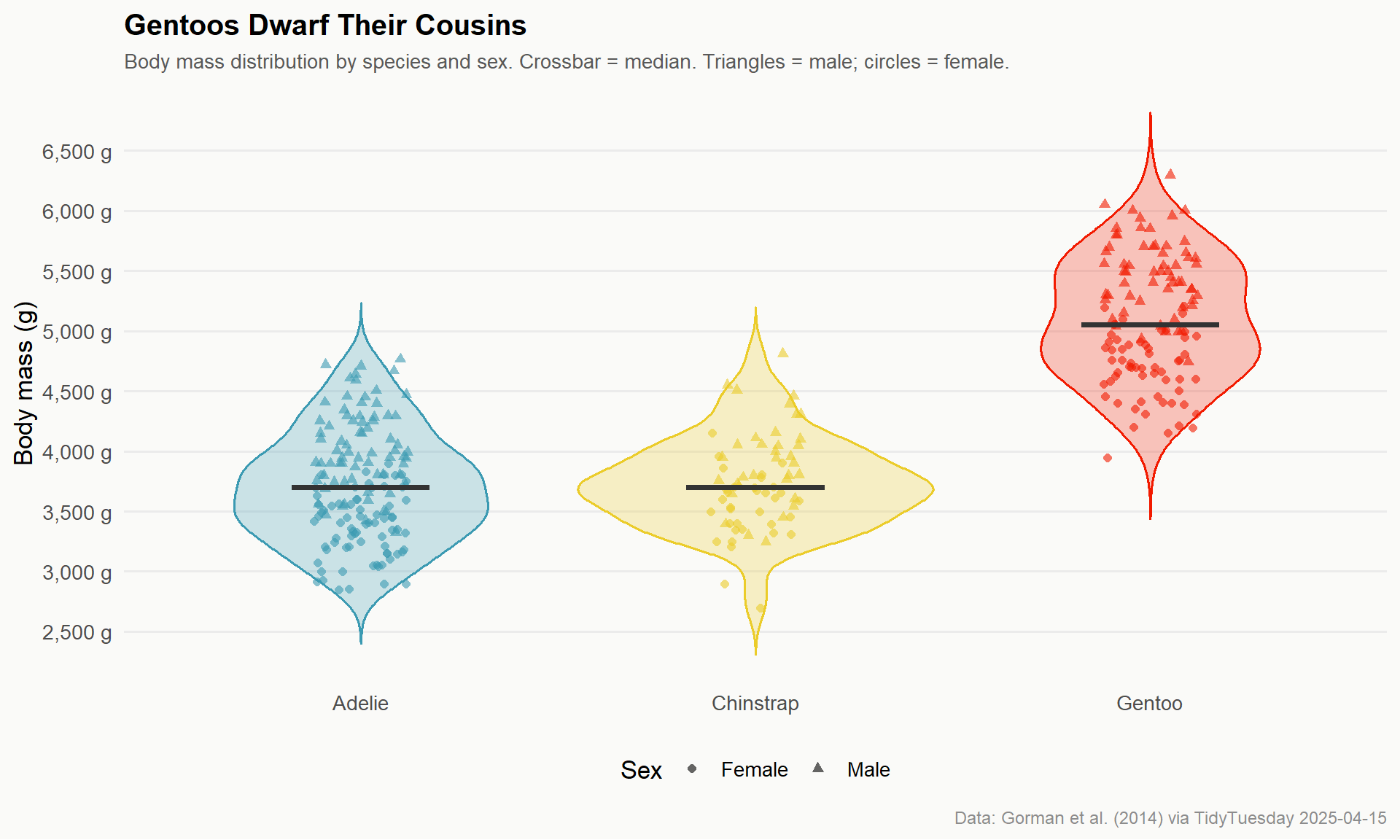
The isotopic data tells us what penguins eat; body mass tells us how big they get. Gentoos, which occupy a higher and more benthic isotopic niche, are also the largest species by a wide margin. Here we look at body mass distributions broken down by species and sex.

# Use the clean dataset for this section
bm_data <- penguins %>%
  filter(!is.na(body_mass_g), !is.na(sex)) %>%
  mutate(
    species = factor(species, levels = c("Adelie", "Chinstrap", "Gentoo")),
    sex     = str_to_title(sex)
  )

cat(sprintf("body mass data: %d rows\n", nrow(bm_data)))

body mass data: 333 rows

stopifnot("Body mass data is empty" = nrow(bm_data) > 0)

bm_data %>% count(species, sex)

    species    sex  n
1    Adelie Female 73
2    Adelie   Male 73
3 Chinstrap Female 34
4 Chinstrap   Male 34
5    Gentoo Female 58
6    Gentoo   Male 61

p_bm <- ggplot2::ggplot(
  bm_data,
  ggplot2::aes(x = species, y = body_mass_g, color = species, fill = species)
) +
  ggplot2::geom_violin(alpha = 0.25, trim = FALSE, linewidth = 0.6) +
  ggplot2::geom_jitter(
    ggplot2::aes(shape = sex),
    width = 0.12, alpha = 0.60, size = 1.8
  ) +
  ggplot2::stat_summary(
    fun = median, geom = "crossbar",
    width = 0.35, linewidth = 0.7, fatten = 2,
    color = "grey20"
  ) +
  ggplot2::scale_color_manual(values = species_colors, guide = "none") +
  ggplot2::scale_fill_manual(values  = species_colors, guide = "none") +
  ggplot2::scale_shape_manual(values = c("Female" = 16, "Male" = 17)) +
  ggplot2::scale_y_continuous(
    labels = scales::label_comma(suffix = " g"),
    breaks = seq(2500, 6500, 500)
  ) +
  ggplot2::labs(
    title    = "Gentoos Dwarf Their Cousins",
    subtitle = "Body mass distribution by species and sex. Crossbar = median. Triangles = male; circles = female.",
    x        = NULL,
    y        = "Body mass (g)",
    shape    = "Sex",
    caption  = "Data: Gorman et al. (2014) via TidyTuesday 2025-04-15"
  ) +
  ggplot2::theme_minimal(base_size = 13) +
  ggplot2::theme(
    plot.title       = ggplot2::element_text(face = "bold", size = 15),
    plot.subtitle    = ggplot2::element_text(color = "grey35", size = 10.5),
    plot.caption     = ggplot2::element_text(color = "grey55", size = 9),
    panel.grid.minor = ggplot2::element_blank(),
    panel.grid.major.x = ggplot2::element_blank(),
    plot.background  = ggplot2::element_rect(fill = "#FAFAF8", color = NA),
    panel.background = ggplot2::element_rect(fill = "#FAFAF8", color = NA),
    legend.position  = "bottom"
  )

p_bm

Palette Log Update

palette_log_path <- here::here("posts", "palette-log.csv")
palette_log      <- read.csv(palette_log_path)

new_entry <- data.frame(
  post_date = "2025-04-15",
  palette   = "Zissou1",
  package   = "wesanderson",
  type      = "discrete"
)

# Only append if this post_date + palette combo isn't already logged
if (!any(palette_log$post_date == new_entry$post_date &
         palette_log$palette   == new_entry$palette)) {
  write.table(
    new_entry,
    palette_log_path,
    append = TRUE, sep = ",", row.names = FALSE, col.names = FALSE
  )
  cat("Palette logged: wesanderson::Zissou1\n")
} else {
  cat("Palette already logged — skipping.\n")
}

Final thoughts and takeaways

The Palmer Penguins dataset is routinely analyzed through bill morphology — the famous length-vs-depth scatter is practically the “Hello, World!” of data visualization. But the raw dataset’s isotope measurements offer a genuinely richer story, one that connects measurement to mechanism.

The δ¹³C signal is the most striking finding: Gentoo penguins occupy a meaningfully different carbon niche from their Pygoscelis relatives. Their less negative δ¹³C (≈ −25.5‰ vs. ≈ −26.5 to −27‰ for Adelie and Chinstrap) is consistent with field studies showing Gentoos are more flexible foragers, diving deeper and targeting fish alongside krill. This dietary breadth may partly explain why Gentoos have expanded their range more successfully under current climate-driven changes to Antarctic sea ice — when krill become patchier, fish remain available.

Adelie and Chinstrap penguins sit in nearly overlapping isotopic space, reflecting their shared krill specialization. Their δ¹⁵N separation is subtle but real, suggesting minor differences in trophic level despite similar carbon sources.

The body mass data hammers the point home: Gentoos aren’t just ecologically distinct — they’re physically in a different league, topping out near 6,300 g while Adelie and Chinstrap overlap almost completely between 3,000–4,750 g. Sexual dimorphism (males heavier than females) is visible in all three species but most pronounced in Gentoos.

Caveats: Isotope values reflect conditions at the time of feather or blood synthesis, and measurements in this dataset come from tissue samples collected at capture. Individual variation within species is substantial, and the 3-year window (2007–2009) may not capture longer-term dietary shifts. Still, the species-level signal is clear and statistically robust.

One final note: with datasets::penguins now in base R 4.5.0, this dataset has officially graduated from “the tidyverse’s iris replacement” to part of the canonical R distribution. Future R learners will encounter these three species before they ever install a package — which means the penguin ecology behind the numbers is worth understanding in depth.