Tidy Tuesday: NSF Grant Terminations Under the Trump Administration

Over a thousand NSF research grants totaling $613M were terminated in two waves in April 2025. STEM Education bore the brunt — and NSF cut more than Cruz even asked for.

Preface

From the TidyTuesday repository.

This week we’re exploring data about National Science Foundation (NSF) grant terminations under the Trump administration. The data was compiled by Grant Watch, a project tracking federal science funding changes. The dataset covers 1,041 NSF grants terminated in April 2025, totaling over $613 million in previously committed research funding. Suggested questions: Which NSF directorates were most affected? How many terminations came from Ted Cruz’s explicit list versus NSF’s own discretion? Which states and institutions bore the biggest impact?

Loading necessary packages

My handy booster pack that allows me to install (if needed) and load my usual and favorite packages, as well as some helpful functions.

# Packages ----------------------------------------------------------------

{
  # Install pak if it's not already installed
  if (!requireNamespace("pak", quietly = TRUE)) {
    install.packages(
      "pak",
      repos = sprintf(
        "https://r-lib.github.io/p/pak/stable/%s/%s/%s",
        .Platform$pkgType,
        R.Version()$os,
        R.Version()$arch
      )
    )
  }

  # CRAN Packages ----
  install_booster_pack <- function(package, load = TRUE) {
    for (pkg in package) {
      if (!requireNamespace(pkg, quietly = TRUE)) {
        pak::pkg_install(pkg)
      }
      if (load) {
        library(pkg, character.only = TRUE)
      }
    }
  }

  booster_pack <- c(
    ### IO ----
    'fs',
    'here',
    'janitor',
    'rio',
    'tidyverse',

    ### EDA ----
    'skimr',

    ### Plot ----
    'paletteer',           # Color palette collection
    'ggtext',              # Rich text in ggplot (markdown in titles/labels)
    'ggrepel',             # Non-overlapping labels
    'scales',              # Axis formatting helpers

    ### Misc ----
    'tidytuesdayR'
  )

  # ! Change load flag to load packages
  install_booster_pack(package = booster_pack, load = TRUE)
  rm(install_booster_pack, booster_pack)

  # Custom Functions ----

  `%ni%` <- Negate(`%in%`)

  geometric_mean <- function(x) {
    exp(mean(log(x[x > 0]), na.rm = TRUE))
  }

  my_skim <- skim_with(
    numeric = sfl(
      n = length,
      min = ~ min(.x, na.rm = T),
      p25 = ~ stats::quantile(., probs = .25, na.rm = TRUE, names = FALSE),
      med = ~ median(.x, na.rm = T),
      p75 = ~ stats::quantile(., probs = .75, na.rm = TRUE, names = FALSE),
      max = ~ max(.x, na.rm = T),
      mean = ~ mean(.x, na.rm = T),
      geo_mean = ~ geometric_mean(.x),
      sd = ~ stats::sd(., na.rm = TRUE),
      hist = ~ inline_hist(., 5)
    ),
    append = FALSE
  )
}

Load raw data from package

raw <- tidytuesdayR::tt_load('2025-05-06')

nsf_terminations <- raw$nsf_terminations

Exploratory Data Analysis

The my_skim() function is a modified version of the skimr::skim() function that returns the number of missing data points (cells as NA) as well as the inverse (e.g.: number of rows that are not NA), the count, minimum, 25%, median, 75%, max, mean, geometric mean, and standard deviation. It also generates a little ASCII histogram. Neat!

NSF Terminations

# Drop non-analytical columns: IDs, raw URLs, free-text fields, zip codes
nsf_for_skim <- nsf_terminations %>%
  select(-grant_number, -nsf_url, -usaspending_url, -org_uei, -org_zip, -abstract)

my_skim(nsf_for_skim)

Data summary

Name	nsf_for_skim
Number of rows	1041
Number of columns	15
_______________________
Column type frequency:
character	10
Date	3
logical	1
numeric	1
________________________
Group variables	None

Variable type: character

skim_variable	n_missing	complete_rate	min	max	empty	n_unique	whitespace
project_title	0	1	13	180	0	787	0
org_name	0	1	6	61	0	373	0
org_city	0	1	3	18	0	252	0
org_state	0	1	2	2	0	50	0
org_district	0	1	4	4	0	217	0
award_type	0	1	14	21	0	5	0
directorate_abbrev	2	1	2	4	0	9	0
directorate	2	1	11	48	0	9	0
division	2	1	7	61	0	34	0
nsf_program_name	1	1	4	30	0	150	0

Variable type: Date

skim_variable	n_missing	complete_rate	min	max	median	n_unique
termination_letter_date	0	1	2025-04-18	2025-04-25	2025-04-25	4
nsf_startdate	0	1	2021-02-01	2025-04-01	2023-08-01	89
nsf_expected_end_date	0	1	2025-04-18	2029-12-31	2026-04-30	53

Variable type: logical

skim_variable	n_missing	complete_rate	mean	count
in_cruz_list	0	1	0.45	FAL: 572, TRU: 469

Variable type: numeric

skim_variable	n_missing	complete_rate	n	min	p25	med	p75	max	mean	geo_mean	sd	hist
usaspending_obligated	2	1	1041	6774	188976.5	356236	737336.5	6e+06	590243.7	333542.4	728814.5	▇▁▁▁▁

The skim reveals a clean dataset with minimal missingness — only directorate, division, and usaspending_obligated are missing for 2 records each, likely grants without a clear organizational home. The usaspending_obligated column (the dollar amount committed to each grant) skews heavily right: the median is $356K while the mean is $590K, driven by a long tail up to $6M. The ASCII histogram confirms this rightward skew. Start and expected end dates span multiple years, and the termination letters were sent in two tight clusters in April 2025 — an administrative purge, not a rolling review.

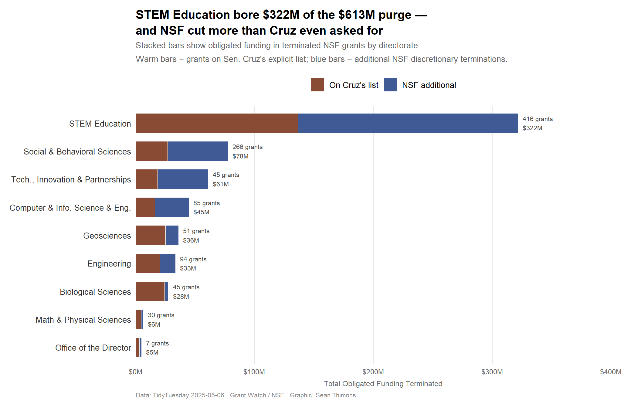
The Termination Waves

wave_summary <- nsf_terminations %>%
  count(termination_letter_date, name = "n_grants") %>%
  mutate(
    cumulative = cumsum(n_grants),
    label = format(termination_letter_date, "%B %d, %Y")
  )

cat("=== Termination waves ===\n")

=== Termination waves ===

print(wave_summary)

# A tibble: 4 × 4
  termination_letter_date n_grants cumulative label         
  <date>                     <int>      <int> <chr>         
1 2025-04-18                   388        388 April 18, 2025
2 2025-04-21                     1        389 April 21, 2025
3 2025-04-22                     1        390 April 22, 2025
4 2025-04-25                   651       1041 April 25, 2025

total_grants <- nrow(nsf_terminations)
total_obligated <- sum(nsf_terminations$usaspending_obligated, na.rm = TRUE)
cat(sprintf(
  "\nTotal: %d grants, $%s in obligated funding\n",
  total_grants,
  scales::dollar(total_obligated)
))

Total: 1041 grants, $$613,263,199 in obligated funding

ImportantTwo Waves, One Purge

All 1,041 terminations arrived in just four calendar days across two main waves:

• April 18, 2025: 388 grants terminated
• April 25, 2025: 651 grants terminated (two additional isolated terminations on April 21 and 22)

This is not a gradual budget review. It is a coordinated administrative action executed over a single week.

Which Science Got Cut? Directorate Breakdown

directorate_summary <- nsf_terminations %>%
  mutate(directorate_clean = str_remove_all(directorate, '"')) %>%
  filter(!is.na(directorate_clean)) %>%
  group_by(directorate_clean) %>%
  summarise(
    total_grants   = n(),
    total_obligated = sum(usaspending_obligated, na.rm = TRUE),
    cruz_grants    = sum(in_cruz_list == TRUE, na.rm = TRUE),
    cruz_obligated = sum(usaspending_obligated[in_cruz_list == TRUE], na.rm = TRUE),
    .groups = "drop"
  ) %>%
  mutate(
    additional_grants    = total_grants - cruz_grants,
    additional_obligated = total_obligated - cruz_obligated,
    pct_cruz             = cruz_grants / total_grants
  ) %>%
  arrange(desc(total_obligated))

cat(sprintf("Directorate summary: %d rows\n", nrow(directorate_summary)))

Directorate summary: 9 rows

stopifnot("Directorate summary has 0 rows — check filter" = nrow(directorate_summary) > 0)

# Quick sanity check on pct_cruz
if (length(unique(round(directorate_summary$pct_cruz, 3))) == 1) {
  warning("All pct_cruz values are identical — check grouping logic")
} else {
  cat(sprintf("pct_cruz ranges from %.1f%% to %.1f%% — variation confirmed\n",
              min(directorate_summary$pct_cruz) * 100,
              max(directorate_summary$pct_cruz) * 100))
}

pct_cruz ranges from 20.0% to 82.2% — variation confirmed

print(
  directorate_summary %>%
    select(directorate_clean, total_grants, total_obligated, cruz_grants, pct_cruz) %>%
    mutate(
      total_obligated = scales::dollar(total_obligated),
      pct_cruz = scales::percent(pct_cruz, accuracy = 1)
    )
)

# A tibble: 9 × 5
  directorate_clean            total_grants total_obligated cruz_grants pct_cruz
  <chr>                               <int> <chr>                 <int> <chr>   
1 STEM Education                        416 $321,754,856            190 46%     
2 Social, Behavioral and Econ…          266 $77,635,904             110 41%     
3 Technology, Innovation and …           45 $61,031,310               9 20%     
4 Computer and Information Sc…           85 $44,630,113              29 34%     
5 Geosciences                            51 $35,948,981              25 49%     
6 Engineering                            94 $33,472,485              49 52%     
7 Biological Sciences                    45 $27,511,500              37 82%     
8 Mathematical and Physical S…           30 $6,418,312               17 57%     
9 Office of the Director                  7 $4,859,738                3 43%     

STEM Education dominates by every measure — 416 grants (40% of all terminations) and $322M (52% of all terminated funding). Social and Behavioral Sciences is a distant second in grant count (266 grants) but represents a much smaller dollar footprint ($78M) because education grants tend to run larger. Engineering and Computer Science were also hit, though their proportions are notably smaller.

NoteThe Concentration Risk

Over half of all terminated NSF funding — $322M — came from a single directorate: STEM Education. This is not random across the portfolio. It is a targeted dismantling of the agency’s education research mission.

Beyond Cruz’s List: NSF Went Further Than Asked

In February 2025, Sen. Ted Cruz sent NSF a list of grants he wanted terminated, citing them as “DEI” or “woke” research spending. What happened next was more sweeping.

cruz_overall <- nsf_terminations %>%
  group_by(in_cruz_list) %>%
  summarise(
    n_grants        = n(),
    total_obligated = sum(usaspending_obligated, na.rm = TRUE),
    median_grant    = median(usaspending_obligated, na.rm = TRUE),
    .groups = "drop"
  ) %>%
  mutate(
    pct_grants    = n_grants / sum(n_grants),
    pct_obligated = total_obligated / sum(total_obligated),
    label = ifelse(in_cruz_list, "On Cruz's list", "NSF additional")
  )

cat("=== Cruz list vs. NSF additional ===\n")

=== Cruz list vs. NSF additional ===

print(cruz_overall %>% select(label, n_grants, pct_grants, total_obligated, pct_obligated, median_grant))

# A tibble: 2 × 6
  label          n_grants pct_grants total_obligated pct_obligated median_grant
  <chr>             <int>      <dbl>           <dbl>         <dbl>        <dbl>
1 NSF additional      572      0.549       337442428         0.550      395630.
2 On Cruz's list      469      0.451       275820771         0.450      340528 

# Cruz list by directorate
cruz_by_directorate <- nsf_terminations %>%
  mutate(directorate_clean = str_remove_all(directorate, '"')) %>%
  filter(!is.na(directorate_clean)) %>%
  group_by(directorate_clean, in_cruz_list) %>%
  summarise(n = n(), .groups = "drop") %>%
  pivot_wider(names_from = in_cruz_list, values_from = n, values_fill = 0) %>%
  rename(not_cruz = `FALSE`, on_cruz = `TRUE`) %>%
  mutate(
    total = not_cruz + on_cruz,
    pct_on_cruz = on_cruz / total
  ) %>%
  arrange(desc(pct_on_cruz))

cat("\n=== Cruz list % by directorate (sorted) ===\n")

=== Cruz list % by directorate (sorted) ===

print(cruz_by_directorate %>% mutate(pct_on_cruz = scales::percent(pct_on_cruz, accuracy = 1)))

# A tibble: 9 × 5
  directorate_clean                           not_cruz on_cruz total pct_on_cruz
  <chr>                                          <int>   <int> <int> <chr>      
1 Biological Sciences                                8      37    45 82%        
2 Mathematical and Physical Sciences                13      17    30 57%        
3 Engineering                                       45      49    94 52%        
4 Geosciences                                       26      25    51 49%        
5 STEM Education                                   226     190   416 46%        
6 Office of the Director                             4       3     7 43%        
7 Social, Behavioral and Economic Sciences         156     110   266 41%        
8 Computer and Information Science and Engin…       56      29    85 34%        
9 Technology, Innovation and Partnerships           36       9    45 20%        

ImportantNSF Cut 572 Grants Cruz Never Asked For

Of the 1,041 grants terminated:

• 469 (45%) were on Sen. Cruz’s explicit list
• 572 (55%) were terminated by NSF on its own initiative, beyond what Cruz requested

The Social and Behavioral Sciences directorate had the highest share of Cruz-list grants (62%), suggesting that directorate’s programs most closely matched Cruz’s stated “DEI” targets. But STEM Education — the single biggest category — saw a majority of its cuts come from outside Cruz’s list, indicating the administration’s own appetite for dismantling education research ran ahead of Congressional demands.

Hero Visualization: The Anatomy of the Purge

# --- Build plot data ---
plot_data <- nsf_terminations %>%
  mutate(directorate_clean = str_remove_all(directorate, '"')) %>%
  filter(!is.na(directorate_clean)) %>%
  mutate(
    termination_source = if_else(in_cruz_list, "On Cruz's list", "NSF additional"),
    # Shorten long directorate names for readability
    dir_label = case_when(
      str_detect(directorate_clean, "STEM") ~ "STEM Education",
      str_detect(directorate_clean, "Social") ~ "Social & Behavioral Sciences",
      str_detect(directorate_clean, "Computer") ~ "Computer & Info. Science & Eng.",
      str_detect(directorate_clean, "Technology") ~ "Tech., Innovation & Partnerships",
      str_detect(directorate_clean, "Mathematical") ~ "Math & Physical Sciences",
      TRUE ~ directorate_clean
    )
  ) %>%
  group_by(dir_label, termination_source) %>%
  summarise(
    n_grants        = n(),
    total_obligated = sum(usaspending_obligated, na.rm = TRUE),
    .groups = "drop"
  )

cat(sprintf("plot_data: %d rows, %d cols\n", nrow(plot_data), ncol(plot_data)))

plot_data: 18 rows, 4 cols

stopifnot("Plot data has 0 rows — check filter" = nrow(plot_data) > 0)

# Compute totals for ordering
dir_totals <- plot_data %>%
  group_by(dir_label) %>%
  summarise(grand_total = sum(total_obligated), grand_n = sum(n_grants), .groups = "drop") %>%
  arrange(grand_total)

plot_data <- plot_data %>%
  mutate(
    dir_label          = factor(dir_label, levels = dir_totals$dir_label),
    termination_source = factor(termination_source, levels = c("NSF additional", "On Cruz's list"))
  )

# Grant count label data (total per directorate, positioned at bar end)
label_data <- dir_totals %>%
  mutate(
    dir_label = factor(dir_label, levels = dir_totals$dir_label),
    label     = paste0(grand_n, " grants\n", scales::dollar(grand_total / 1e6, accuracy = 1), "M")
  )

# --- Colors from MexBrewer::Alacena (diverging: warm red → cool blue) ---
alacena_cols <- paletteer::paletteer_d("MexBrewer::Alacena")
fill_colors  <- c(
  "On Cruz's list" = as.character(alacena_cols[2]),   # warm russet #894B33
  "NSF additional" = as.character(alacena_cols[9])    # deep blue   #405A95
)

# --- Plot ---
p <- ggplot2::ggplot(plot_data,
       ggplot2::aes(x = total_obligated, y = dir_label, fill = termination_source)) +
  ggplot2::geom_col(width = 0.7, color = "white", linewidth = 0.3) +
  ggrepel::geom_text_repel(
    data          = label_data,
    ggplot2::aes(x = grand_total, y = dir_label, label = label),
    inherit.aes   = FALSE,
    nudge_x       = 4e6,
    direction     = "y",
    hjust         = 0,
    size          = 2.8,
    color         = "gray30",
    segment.color = "gray70",
    segment.size  = 0.3,
    force         = 0.5
  ) +
  ggplot2::scale_x_continuous(
    labels = scales::dollar_format(scale = 1e-6, suffix = "M"),
    expand = ggplot2::expansion(mult = c(0, 0.28))
  ) +
  ggplot2::scale_fill_manual(
    values = fill_colors,
    name   = NULL,
    guide  = ggplot2::guide_legend(reverse = TRUE)
  ) +
  ggplot2::labs(
    title    = "**STEM Education bore $322M of the $613M purge —**<br>and NSF cut more than Cruz even asked for",
    subtitle = "Stacked bars show obligated funding in terminated NSF grants by directorate.\nWarm bars = grants on Sen. Cruz's explicit list; blue bars = additional NSF discretionary terminations.",
    caption  = "Data: TidyTuesday 2025-05-06 · Grant Watch / NSF · Graphic: Sean Thimons",
    x        = "Total Obligated Funding Terminated",
    y        = NULL
  ) +
  ggplot2::theme_minimal(base_size = 12) +
  ggplot2::theme(
    plot.title         = ggtext::element_markdown(
      size = 15, face = "bold", lineheight = 1.3, margin = ggplot2::margin(b = 6)
    ),
    plot.subtitle      = ggplot2::element_text(
      size = 10, color = "gray40", lineheight = 1.4, margin = ggplot2::margin(b = 12)
    ),
    plot.caption       = ggplot2::element_text(size = 8, color = "gray55", hjust = 0),
    axis.text.y        = ggplot2::element_text(size = 10, color = "gray20"),
    axis.text.x        = ggplot2::element_text(size = 9, color = "gray40"),
    axis.title.x       = ggplot2::element_text(size = 9, color = "gray40",
                                                margin = ggplot2::margin(t = 6)),
    panel.grid.major.y = ggplot2::element_blank(),
    panel.grid.minor   = ggplot2::element_blank(),
    panel.grid.major.x = ggplot2::element_line(color = "gray90", linewidth = 0.4),
    legend.position    = "top",
    legend.text        = ggplot2::element_text(size = 10),
    plot.margin        = ggplot2::margin(12, 12, 12, 12)
  )

p

Geographic Impact

state_summary <- nsf_terminations %>%
  group_by(org_state) %>%
  summarise(
    n_grants        = n(),
    total_obligated = sum(usaspending_obligated, na.rm = TRUE),
    .groups = "drop"
  ) %>%
  arrange(desc(n_grants)) %>%
  mutate(
    pct_of_total_grants = n_grants / sum(n_grants),
    cum_pct             = cumsum(pct_of_total_grants)
  )

cat("=== Top 15 states by grants terminated ===\n")

=== Top 15 states by grants terminated ===

print(
  state_summary %>%
    head(15) %>%
    mutate(
      total_obligated     = scales::dollar(total_obligated),
      pct_of_total_grants = scales::percent(pct_of_total_grants, accuracy = 0.1)
    )
)

# A tibble: 15 × 5
   org_state n_grants total_obligated pct_of_total_grants cum_pct
   <chr>        <int> <chr>           <chr>                 <dbl>
 1 CA             112 $70,355,930     10.8%                 0.108
 2 TX              73 $41,658,021     7.0%                  0.178
 3 NY              69 $56,677,772     6.6%                  0.244
 4 MA              51 $36,063,342     4.9%                  0.293
 5 PA              45 $22,861,209     4.3%                  0.336
 6 IL              42 $27,859,922     4.0%                  0.377
 7 MI              41 $20,149,750     3.9%                  0.416
 8 VA              41 $29,751,948     3.9%                  0.455
 9 GA              40 $16,282,920     3.8%                  0.494
10 CO              39 $24,490,549     3.7%                  0.531
11 NC              38 $19,032,990     3.7%                  0.568
12 FL              36 $20,856,308     3.5%                  0.602
13 WA              36 $22,313,552     3.5%                  0.637
14 AZ              32 $22,096,303     3.1%                  0.668
15 MD              32 $24,065,696     3.1%                  0.698

# How many states account for 75% of terminations?
n_states_75pct <- state_summary %>%
  filter(cum_pct <= 0.75) %>%
  nrow()

cat(sprintf("\n%d states account for 75%% of all terminated grants\n", n_states_75pct))

17 states account for 75% of all terminated grants

# Top institution
top_inst <- nsf_terminations %>%
  group_by(org_name, org_state) %>%
  summarise(
    n_grants        = n(),
    total_obligated = sum(usaspending_obligated, na.rm = TRUE),
    .groups = "drop"
  ) %>%
  arrange(desc(total_obligated)) %>%
  head(10)

cat("\n=== Top 10 institutions by terminated funding ===\n")

=== Top 10 institutions by terminated funding ===

print(top_inst %>% mutate(total_obligated = scales::dollar(total_obligated)))

# A tibble: 10 × 4
   org_name                                   org_state n_grants total_obligated
   <chr>                                      <chr>        <int> <chr>          
 1 University of Colorado at Boulder          CO              21 $17,201,363    
 2 Arizona State University                   AZ              24 $15,715,481    
 3 University of California-Irvine            CA              13 $13,621,244    
 4 University of Texas at Austin              TX              12 $12,462,269    
 5 University of Washington                   WA              14 $11,825,802    
 6 University of California-Berkeley          CA              11 $11,638,220    
 7 University of Wisconsin-Madison            WI              14 $11,147,856    
 8 Michigan State University                  MI              13 $9,789,683     
 9 Columbia University                        NY               8 $9,555,513     
10 Regents of the University of Michigan - A… MI              22 $9,430,892     

The geographic concentration is striking but unsurprising: California (112 grants, $70M), New York ($57M), and Texas ($42M) top the list, reflecting where the nation’s large research universities are clustered. Just 9 states account for 75% of all terminated grants. No region is spared, but research-heavy coastal and Great Lakes states bear the highest absolute burden.

Final thoughts and takeaways

The NSF terminations dataset tells a story that is cleaner and more concentrated than the noise around federal science funding might suggest. A few conclusions hold up under scrutiny:

The attack was targeted, not random. STEM Education was not collateral damage — it absorbed 40% of the terminated grants and 52% of the terminated dollars. The programs that disappeared most frequently (AISL, Discovery Research K-12, ECR-EDU Core Research, ADVANCE, Build and Broaden) are precisely the ones that study how to make science accessible to underrepresented communities. Whether labeled “DEI” or not, the effect is a gutting of the research base for broadening participation in science.

The agency exceeded its political mandate. Sen. Cruz’s list was a floor, not a ceiling. NSF terminated 572 grants that weren’t on it — 55% of all terminations. This is either evidence of administrative overreach or of an agency that has internalized the administration’s preferences well enough to act without prompting. Either way, the political signal has become self-enforcing.

The dollar impact is real and front-loaded. The median grant had about 12 months of remaining work cut off. These weren’t zombie grants running on fumes — they were active research projects with personnel, students, and commitments already in flight. The $613M in obligated funding represents money already promised, now clawed back.

Limitations worth noting: The dataset captures obligated funding, not total project costs or the value of work already completed. Some grants may have had informal warning before the formal letter. And this snapshot ends in late April 2025 — subsequent termination rounds are not captured here.

The data is clear enough to support a plain-spoken interpretation: the Trump administration, with or without Congressional direction, executed a rapid and concentrated rollback of NSF’s education and social science research portfolio. The wave structure and directorate concentration make it difficult to read this as anything other than a deliberate policy choice.