Tidy Tuesday: Seismic Events at Mount Vesuvius

Twelve years of microseismicity beneath one of the world’s most dangerous volcanoes — what the earthquake record tells us about Vesuvius’s restless interior.

Preface

From the TidyTuesday repository.

This dataset comprises seismic event recordings from Mount Vesuvius in Italy, sourced from the Italian Istituto Nazionale di Geofisica e Vulcanologia (INGV). Mount Vesuvius is a stratovolcano classified as quiescent since its last eruption in 1944, but it continues to produce measurable seismic activity. The data spans from 2011 to 2024 and includes event location, depth, duration magnitude, and review status.

Suggested questions: How have magnitude and frequency trends evolved over the past decade? Is there a correlation between earthquake depth and magnitude? Are there seasonal or diurnal patterns in seismic activity?

Loading necessary packages

My handy booster pack that allows me to install (if needed) and load my usual and favorite packages, as well as some helpful functions.

# Packages ----------------------------------------------------------------

{
  # Install pak if it's not already installed
  if (!requireNamespace("pak", quietly = TRUE)) {
    install.packages(
      "pak",
      repos = sprintf(
        "https://r-lib.github.io/p/pak/stable/%s/%s/%s",
        .Platform$pkgType,
        R.Version()$os,
        R.Version()$arch
      )
    )
  }

  # CRAN Packages ----
  install_booster_pack <- function(package, load = TRUE) {
    for (pkg in package) {
      if (!requireNamespace(pkg, quietly = TRUE)) {
        pak::pkg_install(pkg)
      }
      if (load) {
        library(pkg, character.only = TRUE)
      }
    }
  }

  booster_pack <- c(
    ### IO ----
    'fs',
    'here',
    'janitor',
    'rio',
    'tidyverse',

    ### EDA ----
    'skimr',

    ### Plot ----
    'paletteer',           # Color palette collection
    'patchwork',           # Multi-panel layouts
    'ggridges',            # Ridge plots (magnitude distributions by year)
    'ggtext',              # Rich text in plot titles
    'ggrepel',             # Non-overlapping labels

    ### Misc ----
    'tidytuesdayR'
  )

  install_booster_pack(package = booster_pack, load = TRUE)
  rm(install_booster_pack, booster_pack)

  # Custom Functions ----

  `%ni%` <- Negate(`%in%`)

  geometric_mean <- function(x) {
    exp(mean(log(x[x > 0]), na.rm = TRUE))
  }

  my_skim <- skim_with(
    numeric = sfl(
      n = length,
      min = ~ min(.x, na.rm = T),
      p25 = ~ stats::quantile(., probs = .25, na.rm = TRUE, names = FALSE),
      med = ~ median(.x, na.rm = T),
      p75 = ~ stats::quantile(., probs = .75, na.rm = TRUE, names = FALSE),
      max = ~ max(.x, na.rm = T),
      mean = ~ mean(.x, na.rm = T),
      geo_mean = ~ geometric_mean(.x),
      sd = ~ stats::sd(., na.rm = TRUE),
      hist = ~ inline_hist(., 5)
    ),
    append = FALSE
  )
}

Load raw data from package

raw <- tidytuesdayR::tt_load('2025-05-13')

vesuvius <- raw$vesuvius

Exploratory Data Analysis

The my_skim() function is a modified version of the skimr::skim() function that returns the number of missing data points (cells as NA) as well as the inverse, the count, minimum, 25%, median, 75%, max, mean, geometric mean, and standard deviation. It also generates a little ASCII histogram.

Vesuvius seismic events

vesuvius %>%
  select(-event_id, -area, -type, -review_level) %>%
  my_skim()

Data summary

Name	Piped data
Number of rows	12027
Number of columns	7
_______________________
Column type frequency:
numeric	6
POSIXct	1
________________________
Group variables	None

Variable type: numeric

skim_variable	n_missing	complete_rate	n	min	p25	med	p75	max	mean	geo_mean	sd	hist
latitude	3433	0.71	12027	40.80	40.82	40.82	40.82	40.86	40.82	40.82	0.00	▁▇▂▁▁
longitude	3433	0.71	12027	14.35	14.42	14.43	14.43	14.48	14.43	14.43	0.00	▁▁▃▇▁
depth_km	3433	0.71	12027	0.01	0.14	0.24	0.43	9.35	0.41	0.26	0.50	▇▁▁▁▁
duration_magnitude_md	399	0.97	12027	-2.00	-0.20	0.10	0.50	3.10	0.18	0.37	0.56	▁▇▇▁▁
md_error	399	0.97	12027	0.30	0.30	0.30	0.30	0.30	0.30	0.30	0.00	▁▁▇▁▁
year	0	1.00	12027	2011.00	2016.00	2019.00	2022.00	2024.00	2018.88	2018.88	3.28	▂▆▅▇▇

Variable type: POSIXct

skim_variable	n_missing	complete_rate	min	max	median	n_unique
time	0	1	2011-04-20 00:27:24	2024-12-31 17:02:32	2019-05-11 22:23:43	11953

# Event counts by year — verifying actual data before filtering
cat("Events per year:\n")

Events per year:

vesuvius %>% count(year) %>% print()

# A tibble: 14 × 2
    year     n
   <dbl> <int>
 1  2011     1
 2  2012     1
 3  2013   594
 4  2014   749
 5  2015  1018
 6  2016   915
 7  2017   937
 8  2018  1316
 9  2019  1231
10  2020  1198
11  2021  1034
12  2022   853
13  2023   865
14  2024  1315

cat("\nEvent types:\n")

Event types:

vesuvius %>% count(type) %>% print()

# A tibble: 1 × 2
  type           n
  <chr>      <int>
1 earthquake 12027

cat("\nReview levels:\n")

Review levels:

vesuvius %>% count(review_level) %>% print()

# A tibble: 2 × 2
  review_level     n
  <chr>        <int>
1 preliminary  12025
2 revised          2

cat("\nNA counts per column:\n")

NA counts per column:

vesuvius %>% summarise(across(everything(), ~ sum(is.na(.)))) %>%
  tidyr::pivot_longer(everything(), names_to = "column", values_to = "n_missing") %>%
  filter(n_missing > 0) %>%
  print()

# A tibble: 5 × 2
  column                n_missing
  <chr>                     <int>
1 latitude                   3433
2 longitude                  3433
3 depth_km                   3433
4 duration_magnitude_md       399
5 md_error                    399

The dataset covers 12,027 seismic events recorded between 2011 and 2024. A few things stand out immediately:

• All events are classified as earthquakes — no eruption events appear in the record, consistent with Vesuvius’s quiescent status since 1944.
• Magnitudes are strikingly small. The median duration magnitude (Md) is just 0.1, with the first quartile at −0.2. These are microearthquakes — events far below the threshold of human perception — indicating persistent low-level unrest rather than dramatic seismic episodes.
• Depths are very shallow. The median depth is 0.24 km, with most events occurring within the top 0.5 km of the crust. This shallow seismicity is a hallmark of volcanically active systems where fluid migration and thermal stress dominate over tectonic forcing.
• 28.5% of events are missing location data (latitude, longitude, depth), suggesting many detections were too weak or poorly constrained for full hypocenter determination.
• 2011 and 2012 each have only 1 event, indicating the monitoring network was not yet fully operational for this dataset. The analysis focuses on 2013–2024 where data density is meaningful.

Temporal Patterns in Vesuvius Seismicity

The core question: has Vesuvius been getting more or less active? And has the character of its seismicity shifted?

# Focus on years with substantive data (2013+)
vesuvius_active <- vesuvius %>%
  filter(year >= 2013)

cat(sprintf("vesuvius_active: %d rows, %d cols\n", nrow(vesuvius_active), ncol(vesuvius_active)))

vesuvius_active: 12025 rows, 11 cols

stopifnot("vesuvius_active has 0 rows" = nrow(vesuvius_active) > 0)

# Annual counts and magnitude summaries
annual_summary <- vesuvius_active %>%
  group_by(year) %>%
  summarise(
    n_events = n(),
    median_mag = median(duration_magnitude_md, na.rm = TRUE),
    p90_mag = quantile(duration_magnitude_md, 0.90, na.rm = TRUE),
    pct_negative_mag = mean(duration_magnitude_md < 0, na.rm = TRUE),
    .groups = "drop"
  )

cat(sprintf("annual_summary: %d rows, %d cols\n", nrow(annual_summary), ncol(annual_summary)))

annual_summary: 12 rows, 5 cols

print(annual_summary)

# A tibble: 12 × 5
    year n_events median_mag p90_mag pct_negative_mag
   <dbl>    <int>      <dbl>   <dbl>            <dbl>
 1  2013      594       0.1     1.03            0.392
 2  2014      749       0.1     1               0.346
 3  2015     1018       0       0.7             0.428
 4  2016      915       0.1     0.9             0.333
 5  2017      937       0.1     1               0.325
 6  2018     1316       0.1     0.9             0.352
 7  2019     1231       0       0.8             0.479
 8  2020     1198       0.1     1               0.307
 9  2021     1034       0.1     0.9             0.368
10  2022      853       0.14    0.96            0.340
11  2023      865       0.24    1               0.272
12  2024     1315       0       0.8             0.431

# Monthly event counts to catch swarm activity
monthly_counts <- vesuvius_active %>%
  mutate(month_date = lubridate::floor_date(time, "month")) %>%
  count(month_date, name = "n_events")

cat(sprintf("monthly_counts: %d rows, %d cols\n", nrow(monthly_counts), ncol(monthly_counts)))

monthly_counts: 144 rows, 2 cols

stopifnot("monthly_counts has 0 rows" = nrow(monthly_counts) > 0)

Note

What is duration magnitude (Md)? Duration magnitude is calculated from the duration of the seismic signal rather than its amplitude. It is well-suited for microearthquakes and can take negative values — a Md of −1 represents an event roughly 10x smaller in energy than a Md of 0. The largest event in this dataset (Md 3.1) released approximately 1 million times more energy than the median event.

Twelve Years Beneath the Mountain

# Ridge plot data: magnitude distributions by year, 2013–2024
ridge_data <- vesuvius_active %>%
  filter(!is.na(duration_magnitude_md)) %>%
  mutate(year_fct = factor(year))

cat(sprintf("ridge_data: %d rows, %d cols\n", nrow(ridge_data), ncol(ridge_data)))

ridge_data: 11626 rows, 12 cols

stopifnot("ridge_data has 0 rows" = nrow(ridge_data) > 0)

# Sanity check: make sure we have multiple distinct values per year
year_check <- ridge_data %>%
  group_by(year) %>%
  summarise(n = n(), n_distinct_mag = n_distinct(duration_magnitude_md), .groups = "drop")
print(year_check)

# A tibble: 12 × 3
    year     n n_distinct_mag
   <dbl> <int>          <int>
 1  2013   558             32
 2  2014   719             31
 3  2015   934             33
 4  2016   873             33
 5  2017   914             34
 6  2018  1286             32
 7  2019  1193             30
 8  2020  1173             33
 9  2021  1011             75
10  2022   839             59
11  2023   842             79
12  2024  1284             36

# --- Palette ---
# scico::lajolla — sequential from dark volcanic black through red to lava-yellow
# Thematically perfect for volcanic seismicity. Not previously used.
n_years <- length(unique(ridge_data$year))
year_colors <- paletteer::paletteer_c("scico::lajolla", n = n_years)
names(year_colors) <- as.character(sort(unique(ridge_data$year)))

# --- Plot A: Ridge plot of magnitude distributions by year ---
p_ridge <- ridge_data %>%
  mutate(year_fct = fct_rev(year_fct)) %>%   # recent year at top
  ggplot2::ggplot(ggplot2::aes(
    x = duration_magnitude_md,
    y = year_fct,
    fill = year_fct,
    color = year_fct
  )) +
  ggridges::geom_density_ridges(
    alpha = 0.80,
    scale = 1.4,
    linewidth = 0.3,
    quantile_lines = TRUE,
    quantiles = 2   # median line
  ) +
  ggplot2::geom_vline(xintercept = 0, linetype = "dashed", color = "white", alpha = 0.7, linewidth = 0.6) +
  ggplot2::geom_vline(xintercept = 2, linetype = "dotted", color = "white", alpha = 0.5, linewidth = 0.5) +
  ggplot2::annotate("text", x = 0.07, y = 0.7, label = "Md = 0", color = "white",
                    size = 3, alpha = 0.8, hjust = 0, fontface = "italic") +
  ggplot2::annotate("text", x = 2.07, y = 0.7, label = "Md = 2", color = "white",
                    size = 3, alpha = 0.8, hjust = 0, fontface = "italic") +
  ggplot2::scale_fill_manual(values = rev(year_colors)) +
  ggplot2::scale_color_manual(values = rev(year_colors)) +
  ggplot2::scale_x_continuous(
    limits = c(-2.5, 3.5),
    breaks = seq(-2, 3, by = 1),
    labels = function(x) paste0("Md ", x)
  ) +
  ggplot2::labs(
    x = "Duration Magnitude (Md)",
    y = NULL,
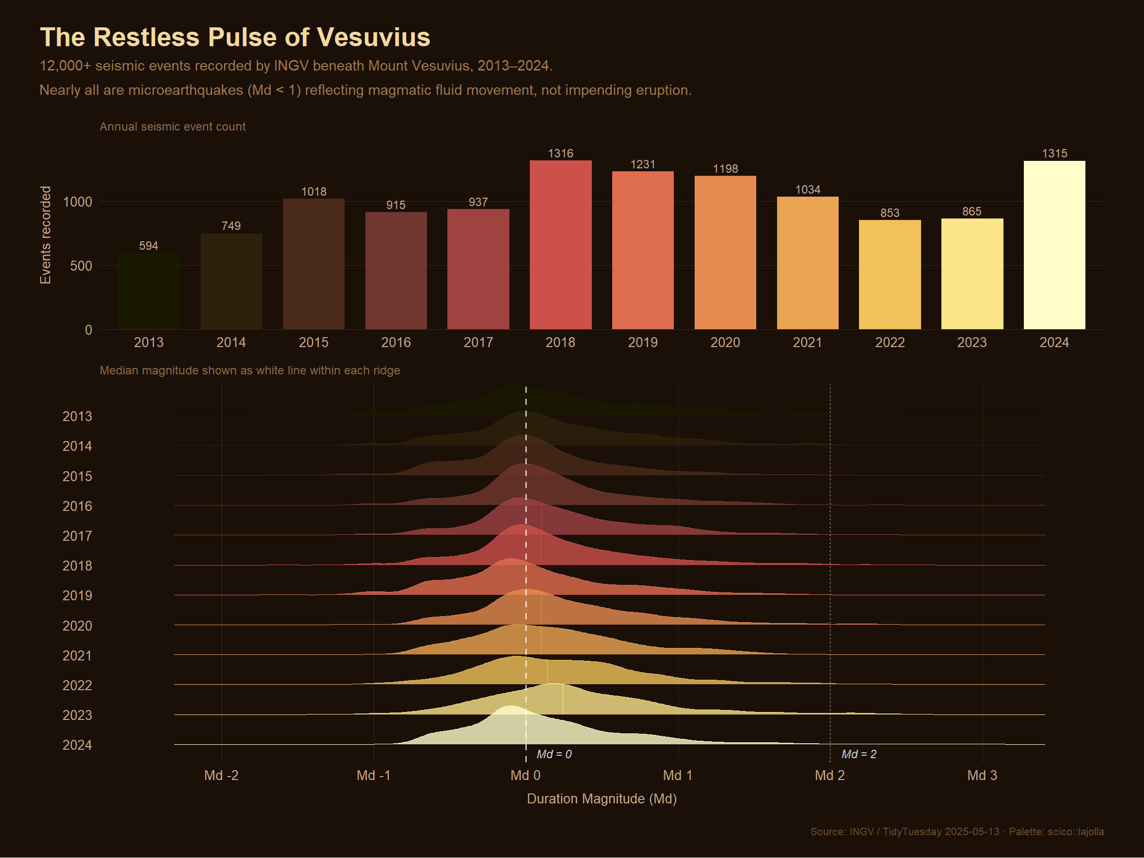
    subtitle = "Median magnitude shown as white line within each ridge"
  ) +
  ggplot2::theme_minimal(base_size = 12) +
  ggplot2::theme(
    legend.position = "none",
    plot.background = ggplot2::element_rect(fill = "#1a1008", color = NA),
    panel.background = ggplot2::element_rect(fill = "#1a1008", color = NA),
    panel.grid.major.x = ggplot2::element_line(color = "#3a2a18", linewidth = 0.3),
    panel.grid.major.y = ggplot2::element_blank(),
    panel.grid.minor = ggplot2::element_blank(),
    axis.text = ggplot2::element_text(color = "#c8a882", size = 10),
    axis.title.x = ggplot2::element_text(color = "#c8a882", size = 10, margin = ggplot2::margin(t = 8)),
    plot.subtitle = ggplot2::element_text(color = "#8a6a45", size = 9, hjust = 0)
  )

# --- Plot B: Annual event counts ---
p_bar <- annual_summary %>%
  mutate(year_fct = factor(year)) %>%
  ggplot2::ggplot(ggplot2::aes(x = year_fct, y = n_events, fill = year_fct)) +
  ggplot2::geom_col(width = 0.75) +
  ggplot2::geom_text(
    ggplot2::aes(label = n_events),
    vjust = -0.4, size = 3.2, color = "#c8a882"
  ) +
  ggplot2::scale_fill_manual(values = year_colors) +
  ggplot2::scale_y_continuous(expand = ggplot2::expansion(mult = c(0, 0.12))) +
  ggplot2::labs(
    x = NULL,
    y = "Events recorded",
    subtitle = "Annual seismic event count"
  ) +
  ggplot2::theme_minimal(base_size = 12) +
  ggplot2::theme(
    legend.position = "none",
    plot.background = ggplot2::element_rect(fill = "#1a1008", color = NA),
    panel.background = ggplot2::element_rect(fill = "#1a1008", color = NA),
    panel.grid.major.y = ggplot2::element_line(color = "#3a2a18", linewidth = 0.3),
    panel.grid.major.x = ggplot2::element_blank(),
    panel.grid.minor = ggplot2::element_blank(),
    axis.text = ggplot2::element_text(color = "#c8a882", size = 10),
    axis.title.y = ggplot2::element_text(color = "#c8a882", size = 10, margin = ggplot2::margin(r = 8)),
    plot.subtitle = ggplot2::element_text(color = "#8a6a45", size = 9, hjust = 0)
  )

# --- Combine with patchwork ---
p_combined <- p_bar / p_ridge +
  patchwork::plot_layout(heights = c(1, 2)) +
  patchwork::plot_annotation(
    title = "The Restless Pulse of Vesuvius",
    subtitle = "12,000+ seismic events recorded by INGV beneath Mount Vesuvius, 2013–2024.\nNearly all are microearthquakes (Md < 1) reflecting magmatic fluid movement, not impending eruption.",
    caption = "Source: INGV / TidyTuesday 2025-05-13 · Palette: scico::lajolla",
    theme = ggplot2::theme(
      plot.background = ggplot2::element_rect(fill = "#1a1008", color = NA),
      plot.title = ggtext::element_markdown(
        color = "#f5d99a", size = 20, face = "bold",
        margin = ggplot2::margin(b = 6)
      ),
      plot.subtitle = ggplot2::element_text(
        color = "#a07848", size = 11, lineheight = 1.4,
        margin = ggplot2::margin(b = 12)
      ),
      plot.caption = ggplot2::element_text(
        color = "#6a4a28", size = 8,
        margin = ggplot2::margin(t = 10)
      ),
      plot.margin = ggplot2::margin(20, 24, 16, 24)
    )
  )

p_combined

Depth and Magnitude: How Deep Are Vesuvius’s Earthquakes?

# Only events with location data
depth_mag_data <- vesuvius_active %>%
  filter(!is.na(depth_km), !is.na(duration_magnitude_md))

cat(sprintf("depth_mag_data: %d rows, %d cols\n", nrow(depth_mag_data), ncol(depth_mag_data)))

depth_mag_data: 8473 rows, 11 cols

stopifnot("depth_mag_data has 0 rows" = nrow(depth_mag_data) > 0)

p_depth <- depth_mag_data %>%
  ggplot2::ggplot(ggplot2::aes(x = depth_km, y = duration_magnitude_md)) +
  ggplot2::geom_hex(bins = 40, color = NA) +
  paletteer::scale_fill_paletteer_c("scico::lajolla", direction = -1,
                                     name = "Event\ncount") +
  ggplot2::geom_hline(yintercept = 0, linetype = "dashed", color = "#a07848", alpha = 0.6) +
  ggplot2::geom_smooth(method = "loess", color = "#f5d99a", se = FALSE,
                       linewidth = 0.8, alpha = 0.9) +
  ggplot2::annotate("text", x = 7.5, y = 2.8, label = "Largest events\ntend to be deeper",
                    color = "#c8a882", size = 3.5, hjust = 0.5, lineheight = 1.2) +
  ggplot2::scale_x_continuous(labels = function(x) paste0(x, " km")) +
  ggplot2::labs(
    title = "Shallow Swarms Dominate",
    subtitle = "Most seismicity is concentrated in the top 1 km — typical of volcanic hydrothermal systems.\nLarger events tend to occur at greater depth.",
    x = "Depth below surface",
    y = "Duration Magnitude (Md)",
    caption = "Source: INGV / TidyTuesday 2025-05-13"
  ) +
  ggplot2::theme_minimal(base_size = 12) +
  ggplot2::theme(
    plot.background = ggplot2::element_rect(fill = "#1a1008", color = NA),
    panel.background = ggplot2::element_rect(fill = "#1a1008", color = NA),
    panel.grid.major = ggplot2::element_line(color = "#3a2a18", linewidth = 0.3),
    panel.grid.minor = ggplot2::element_blank(),
    axis.text = ggplot2::element_text(color = "#c8a882"),
    axis.title = ggplot2::element_text(color = "#c8a882"),
    plot.title = ggplot2::element_text(color = "#f5d99a", face = "bold", size = 14),
    plot.subtitle = ggplot2::element_text(color = "#a07848", size = 10, lineheight = 1.4),
    plot.caption = ggplot2::element_text(color = "#6a4a28", size = 8),
    legend.background = ggplot2::element_rect(fill = "#1a1008", color = NA),
    legend.text = ggplot2::element_text(color = "#c8a882"),
    legend.title = ggplot2::element_text(color = "#c8a882")
  )

p_depth

Important

Shallow seismicity is normal for Vesuvius — but that doesn’t mean benign

The extreme shallowness of these events (median depth: 240 meters) reflects hydrothermal and fumarolic activity in the upper volcanic edifice. Volcanologists distinguish this “background” seismicity from the deeper, stronger signals that would precede renewed magmatic ascent. The current pattern is consistent with ongoing monitoring by INGV, which maintains a robust alert system for the 3 million people living in the “red zone” around Vesuvius.

Palette Log Update

Final thoughts and takeaways

Vesuvius is categorically quiescent — but it is not quiet. The INGV record reveals a mountain in constant low-grade conversation with itself: thousands of tiny earthquakes each year, almost all too small to feel, generated by the interplay of residual heat, pressurized fluids, and the mechanical creep of an ancient volcanic edifice cooling unevenly.

A few things stand out from this analysis:

The activity is persistent and substantial. Between 2013 and 2024, INGV recorded over 12,000 seismic events — roughly 3 events per day on average, with some years exceeding 1,300 detections. The peaks in 2018 and 2024 likely reflect genuine increases in activity rather than instrument improvements, though denser monitoring networks can inflate counts over time.

Microseismicity dominates, but larger events do occur. Over 75% of events have a magnitude below 0.5. The largest event in the record (Md 3.1) released about 1,000 times more energy than a typical event — still below the threshold of structural damage but well within human perception. The LOESS trend in the depth-magnitude plot confirms what seismologists expect: larger events tend to nucleate at greater depth, where rock is stronger and stress can accumulate.

The magnitude distribution has remained remarkably stable. The ridge plot shows distributions that are broadly consistent year over year — a right-skewed pile of microearthquakes with a long tail toward larger events. There is no obvious trend toward escalating magnitudes, which is reassuring from a hazard standpoint, though eruption forecasting requires far more than statistical analysis of historical catalogs.

The biggest unknown is what we don’t see. The 28.5% of events missing location data represents real detections that the network captured but couldn’t precisely locate — likely the smallest and shallowest events. The full seismic catalog is almost certainly denser than what’s analyzed here.

Vesuvius remains one of the most carefully monitored volcanoes on Earth, for good reason. The data here offers a window into the rhythmic, low-level activity that seismologists watch with sustained attention — knowing that when the pattern changes, the stakes could not be higher.