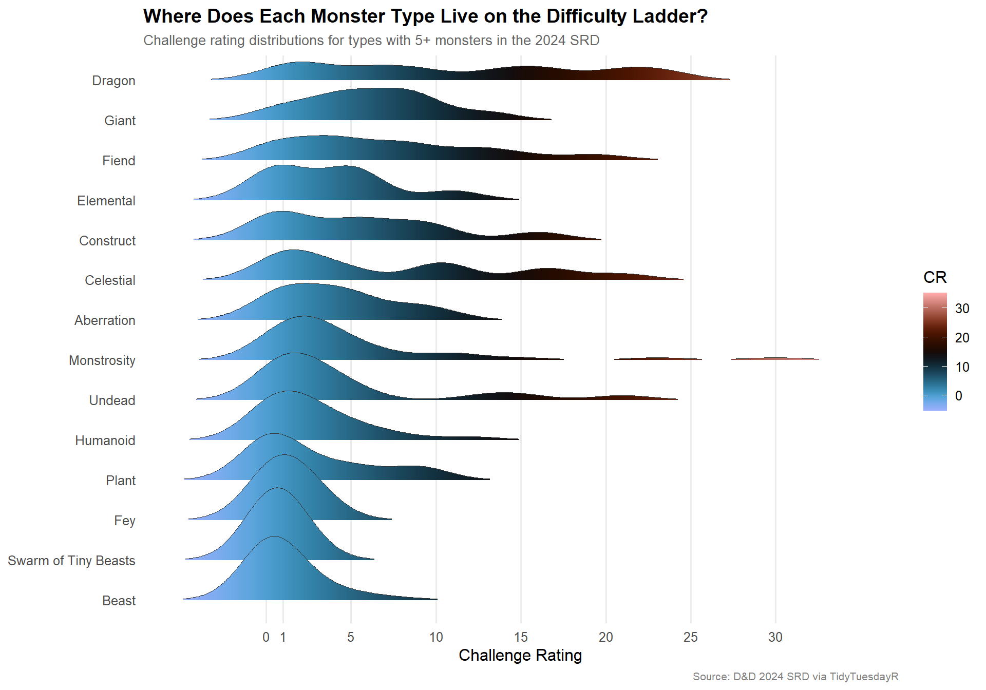
Tidy Tuesday: Dungeons and Dragons Monsters (2024)

Decoding the ability score DNA of D&D 2024 SRD monsters — which creature types hit hardest, cast best, or survive the longest?

Preface

From the TidyTuesday repository.

This week’s data features monsters from the Dungeons & Dragons 2024 System Reference Document (SRD). The SRD is the freely available subset of D&D rules, and the monsters dataset contains creature statistics — ability scores, challenge ratings, hit points, armor class, resistances, languages, and more — for hundreds of creatures drawn from the official ruleset. Suggested questions include: Which monster types exhibit the highest or lowest ability scores? How do monster types vary in challenge rating ranges? Which language enables communication with the most creatures?

Loading necessary packages

My handy booster pack that allows me to install (if needed) and load my usual and favorite packages, as well as some helpful functions.

# Packages ----------------------------------------------------------------

{
  # Install pak if it's not already installed
  if (!requireNamespace("pak", quietly = TRUE)) {
    install.packages(
      "pak",
      repos = sprintf(
        "https://r-lib.github.io/p/pak/stable/%s/%s/%s",
        .Platform$pkgType,
        R.Version()$os,
        R.Version()$arch
      )
    )
  }

  # CRAN Packages ----
  install_booster_pack <- function(package, load = TRUE) {
    for (pkg in package) {
      if (!requireNamespace(pkg, quietly = TRUE)) {
        pak::pkg_install(pkg)
      }
      if (load) {
        library(pkg, character.only = TRUE)
      }
    }
  }

  booster_pack <- c(
    ### IO ----
    'fs',
    'here',
    'janitor',
    'rio',
    'tidyverse',

    ### EDA ----
    'skimr',

    ### Plot ----
    'paletteer',           # Color palette collection
    'patchwork',           # Multi-panel layouts
    'ggtext',              # Rich text in ggplot
    'ggrepel',             # Non-overlapping labels
    'ggridges',            # Ridge/joy plots

    ### Misc ----
    'tidytuesdayR'
  )

  install_booster_pack(package = booster_pack, load = TRUE)
  rm(install_booster_pack, booster_pack)

  # Custom Functions ----

  `%ni%` <- Negate(`%in%`)

  geometric_mean <- function(x) {
    exp(mean(log(x[x > 0]), na.rm = TRUE))
  }

  my_skim <- skim_with(
    numeric = sfl(
      n = length,
      min = ~ min(.x, na.rm = T),
      p25 = ~ stats::quantile(., probs = .25, na.rm = TRUE, names = FALSE),
      med = ~ median(.x, na.rm = T),
      p75 = ~ stats::quantile(., probs = .75, na.rm = TRUE, names = FALSE),
      max = ~ max(.x, na.rm = T),
      mean = ~ mean(.x, na.rm = T),
      geo_mean = ~ geometric_mean(.x),
      sd = ~ stats::sd(., na.rm = TRUE),
      hist = ~ inline_hist(., 5)
    ),
    append = FALSE
  )
}

Load raw data from package

raw <- tidytuesdayR::tt_load('2025-05-27')

monsters <- raw$monsters

Exploratory Data Analysis

The my_skim() function is a modified version of the skimr::skim() function that returns the number of missing data points (cells as NA) as well as the inverse (e.g.: number of rows that are not NA), the count, minimum, 25%, median, 75%, max, mean, geometric mean, and standard deviation. It also generates a little ASCII histogram. Neat!

Monsters

# First, examine the raw structure
glimpse(monsters)

Rows: 330
Columns: 33
$ name              <chr> "Aboleth", "Air Elemental", "Animated Armor", "Anima…
$ category          <chr> "Aboleth", "Air Elemental", "Animated Objects", "Ani…
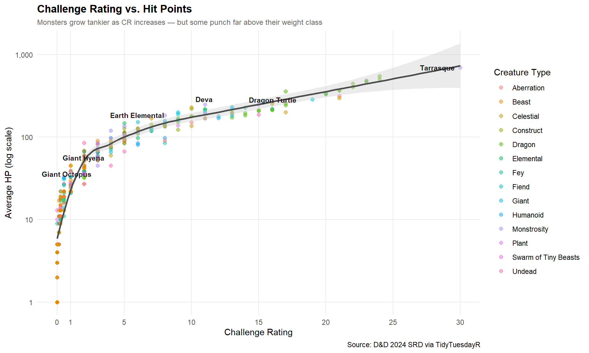
$ cr                <dbl> 10.000, 5.000, 1.000, 0.250, 2.000, 2.000, 8.000, 0.…
$ size              <chr> "Large", "Large", "Medium", "Small", "Large", "Large…
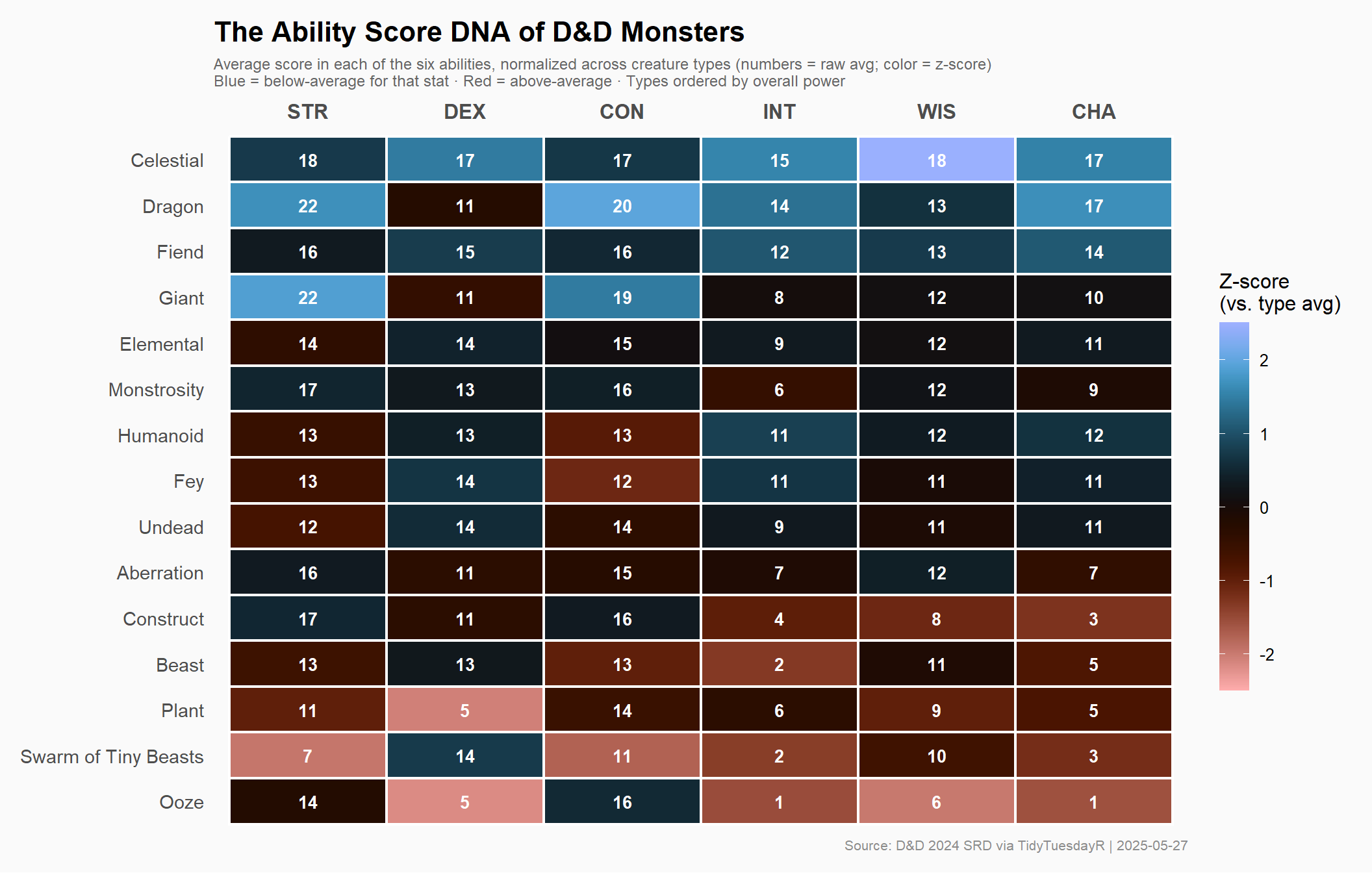
$ type              <chr> "Aberration", "Elemental", "Construct", "Construct",…
$ descriptive_tags  <chr> NA, NA, NA, NA, NA, NA, NA, NA, NA, NA, NA, "Demon",…
$ alignment         <chr> "Lawful Evil", "Neutral", "Unaligned", "Unaligned", …
$ ac                <dbl> 17, 15, 18, 17, 12, 14, 16, 9, 13, 11, 17, 19, 12, 1…
$ initiative        <dbl> 7, 5, 2, 4, 4, 0, 10, -1, -2, 1, 1, 14, 1, 3, 3, -1,…
$ hp                <chr> "150 (20d10 + 40)", "90 (12d10 + 24)", "33 (6d8 + 6)…
$ hp_number         <dbl> 150, 90, 33, 14, 27, 45, 97, 10, 59, 19, 39, 287, 11…
$ speed             <chr> "Speed 10 ft., Swim 40 ft.", "Speed 10 ft., Fly 90 f…
$ speed_base_number <dbl> 10, 10, 25, 5, 10, 30, 30, 20, 20, 50, 30, 40, 30, 3…
$ str               <dbl> 21, 14, 14, 12, 17, 17, 11, 3, 19, 14, 17, 26, 11, 1…
$ dex               <dbl> 9, 20, 11, 15, 14, 11, 18, 8, 6, 12, 12, 15, 12, 16,…
$ con               <dbl> 15, 14, 13, 11, 10, 14, 14, 11, 15, 12, 15, 22, 12, …
$ int               <dbl> 18, 6, 1, 1, 1, 1, 16, 10, 10, 2, 12, 20, 10, 14, 12…
$ wis               <dbl> 15, 10, 3, 5, 3, 13, 11, 10, 10, 10, 13, 16, 10, 11,…
$ cha               <dbl> 18, 6, 1, 1, 1, 6, 10, 6, 7, 5, 10, 22, 10, 14, 14, …
$ str_save          <dbl> 5, 2, 2, 1, 3, 3, 0, -4, 4, 2, 3, 8, 0, 4, 6, 3, 5, …
$ dex_save          <dbl> 3, 5, 0, 4, 2, 0, 7, -1, -2, 1, 1, 2, 1, 5, 3, -1, 2…
$ con_save          <dbl> 6, 2, 1, 0, 0, 2, 2, 0, 2, 1, 4, 12, 1, 2, 7, 2, 4, …
$ int_save          <dbl> 8, -2, -5, -5, -5, -5, 6, 0, 0, -4, 1, 5, 0, 2, 1, -…
$ wis_save          <dbl> 6, 0, -4, -3, -4, 1, 0, 0, 0, 0, 1, 9, 0, 2, 5, -1, …
$ cha_save          <dbl> 4, -2, -5, -5, -5, -2, 0, -2, -2, -3, 0, 6, 0, 2, 5,…
$ skills            <chr> "History +12, Perception +10", NA, NA, NA, NA, NA, "…
$ resistances       <chr> NA, "Bludgeoning, Lightning, Piercing, Slashing", NA…
$ vulnerabilities   <chr> NA, NA, NA, NA, NA, NA, NA, "Fire", "Fire", NA, NA, …
$ immunities        <chr> NA, "Poison, Thunder; Exhaustion, Grappled, Paralyze…
$ gear              <chr> NA, NA, NA, NA, NA, NA, "Light Crossbow, Shortsword,…
$ senses            <chr> "Darkvision 120 ft.; Passive Perception 20", "Darkvi…
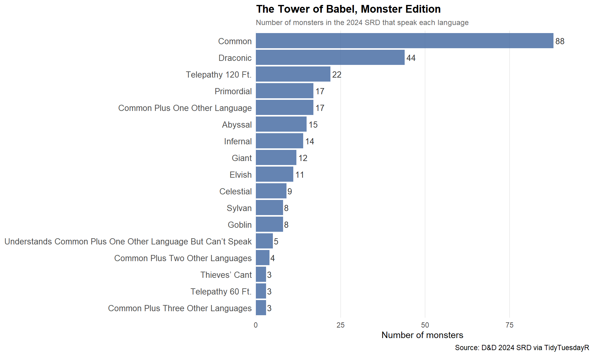
$ languages         <chr> "Deep Speech; telepathy 120 ft.", "Primordial (Auran…
$ full_text         <chr> "Aboleth\nLarge Aberration, Lawful Evil\nAC 17\t\t  …

# Examine categorical distributions
cat("=== Monster Types ===\n")

=== Monster Types ===

monsters %>% count(type, sort = TRUE) %>% print(n = 20)

# A tibble: 16 × 2
   type                     n
   <chr>                <int>
 1 Beast                   84
 2 Dragon                  45
 3 Monstrosity             37
 4 Fiend                   29
 5 Humanoid                26
 6 Undead                  18
 7 Elemental               17
 8 Fey                     15
 9 Celestial               13
10 Construct               10
11 Giant                   10
12 Aberration               9
13 Plant                    6
14 Swarm of Tiny Beasts     6
15 Ooze                     4
16 Swarm of Tiny Undead     1

cat("\n=== Monster Sizes ===\n")

=== Monster Sizes ===

monsters %>% count(size, sort = TRUE)

# A tibble: 7 × 2
  size                n
  <chr>           <int>
1 Large             107
2 Medium             90
3 Medium or Small    36
4 Huge               34
5 Tiny               25
6 Small              23
7 Gargantuan         15

cat("\n=== Challenge Rating Distribution ===\n")

=== Challenge Rating Distribution ===

monsters %>% count(cr, sort = FALSE) %>% arrange(cr) %>% print(n = 30)

# A tibble: 28 × 2
       cr     n
    <dbl> <int>
 1  0        29
 2  0.125    19
 3  0.25     32
 4  0.5      27
 5  1        27
 6  2        42
 7  3        25
 8  4        16
 9  5        25
10  6        11
11  7         6
12  8        10
13  9         8
14 10         6
15 11         7
16 12         2
17 13         6
18 14         3
19 15         4
20 16         5
21 17         4
22 19         1
23 20         3
24 21         4
25 22         2
26 23         3
27 24         2
28 30         1

cat("\n=== Alignment breakdown ===\n")

=== Alignment breakdown ===

monsters %>% count(alignment, sort = TRUE) %>% print(n = 20)

# A tibble: 10 × 2
   alignment           n
   <chr>           <int>
 1 Unaligned         125
 2 Neutral            50
 3 Chaotic Evil       45
 4 Lawful Evil        35
 5 Neutral Evil       28
 6 Lawful Good        20
 7 Chaotic Good       11
 8 Chaotic Neutral     7
 9 Neutral Good        6
10 Lawful Neutral      3

# Profile the six ability scores and CR
monsters %>%
  select(cr, str, dex, con, int, wis, cha) %>%
  my_skim()

Data summary

Name	Piped data
Number of rows	330
Number of columns	7
_______________________
Column type frequency:
numeric	7
________________________
Group variables	None

Variable type: numeric

skim_variable	n_missing	complete_rate	n	min	p25	med	p75	max	mean	geo_mean	sd	hist
cr	0	1	330	0	0.5	2.0	6	30	4.55	2.15	5.80	▇▁▁▁▁
str	0	1	330	1	11.0	16.0	19	30	15.38	13.29	6.52	▂▃▇▃▂
dex	0	1	330	1	10.0	13.0	15	28	12.83	12.31	3.26	▁▅▇▁▁
con	0	1	330	8	12.0	14.5	17	30	15.18	14.59	4.40	▇▇▅▁▁
int	0	1	330	1	2.0	7.0	12	25	7.86	5.51	5.68	▇▅▃▂▁
wis	0	1	330	3	10.0	12.0	13	25	11.82	11.41	2.97	▁▇▇▁▁
cha	0	1	330	1	5.0	8.0	14	30	9.92	7.98	5.97	▇▇▅▂▁

The skim reveals a dataset rich in structure. The six ability scores (STR, DEX, CON, INT, WIS, CHA) each range from single digits up into the low 30s for the mightiest beings. Challenge rating (cr) runs from 0 to 30, with a right-skewed distribution — most monsters cluster at lower CRs, but legendary creatures push all the way to the ceiling. There is relatively little missingness in the core numeric columns, making this a clean dataset for cross-type comparison.

Note

A quick D&D primer: The six ability scores define a creature’s fundamental capabilities. Strength (STR) determines physical power, Dexterity (DEX) covers agility and reflexes, Constitution (CON) governs endurance and hit points, Intelligence (INT) reflects reasoning and memory, Wisdom (WIS) covers perception and willpower, and Charisma (CHA) captures personality and force of presence. An “average” human has 10–11 in each score; scores above 20 are superhuman, and 30 is the theoretical maximum.

# Parse numeric values from character columns (HP and AC contain dice notation)
monsters_clean <- monsters %>%
  janitor::clean_names() %>%
  mutate(
    # Extract the flat numeric portion from HP strings like "52 (8d10 + 8)"
    hp_avg    = as.numeric(str_extract(hp, "^\\d+")),
    # Extract the base AC value from strings like "17 (natural armor)"
    ac_num    = as.numeric(str_extract(ac, "^\\d+")),
    # Convert CR fractions (already numeric as double per the data dictionary)
    cr_num    = as.numeric(cr)
  )

cat(sprintf("monsters_clean: %d rows, %d cols\n",
            nrow(monsters_clean), ncol(monsters_clean)))

monsters_clean: 330 rows, 36 cols

cat(sprintf("HP parsed successfully for %d/%d rows\n",
            sum(!is.na(monsters_clean$hp_avg)), nrow(monsters_clean)))

HP parsed successfully for 330/330 rows

cat(sprintf("AC parsed successfully for %d/%d rows\n",
            sum(!is.na(monsters_clean$ac_num)), nrow(monsters_clean)))

AC parsed successfully for 330/330 rows

The Ability Score DNA of Monster Types

Every D&D creature type has a characteristic “stat fingerprint” — the composite profile of its six ability scores relative to the monster population as a whole. Beasts are physical hunters; Fey rely on nimbleness and charm; undead lack biological vitality but often possess eerie willpower. Let’s make those patterns explicit.

Computing normalized ability score profiles

# Compute average ability scores per type, then z-score each ability
# across all types so we can compare apples to apples
ability_profile <- monsters_clean %>%
  group_by(type) %>%
  summarise(
    STR  = mean(str, na.rm = TRUE),
    DEX  = mean(dex, na.rm = TRUE),
    CON  = mean(con, na.rm = TRUE),
    INT  = mean(int, na.rm = TRUE),
    WIS  = mean(wis, na.rm = TRUE),
    CHA  = mean(cha, na.rm = TRUE),
    n    = n(),
    .groups = "drop"
  ) %>%
  # Only include types with at least 3 monsters for stability
  filter(n >= 3) %>%
  pivot_longer(cols = STR:CHA, names_to = "ability", values_to = "mean_score") %>%
  group_by(ability) %>%
  mutate(z_score = (mean_score - mean(mean_score)) / sd(mean_score)) %>%
  ungroup()

# Integrity check
cat(sprintf("ability_profile: %d rows, %d cols\n",
            nrow(ability_profile), ncol(ability_profile)))

ability_profile: 90 rows, 5 cols

stopifnot(
  "Plot data has 0 rows — check filter values" = nrow(ability_profile) > 0
)

# Sanity check: z-scores should have mean ~0 per ability group
ability_profile %>%
  group_by(ability) %>%
  summarise(mean_z = round(mean(z_score), 8), sd_z = round(sd(z_score), 4))

# A tibble: 6 × 3
  ability mean_z  sd_z
  <chr>    <dbl> <dbl>
1 CHA          0     1
2 CON          0     1
3 DEX          0     1
4 INT          0     1
5 STR          0     1
6 WIS          0     1

# Challenge rating stats by type
cr_by_type <- monsters_clean %>%
  filter(!is.na(cr_num)) %>%
  group_by(type) %>%
  summarise(
    n         = n(),
    median_cr = median(cr_num),
    mean_cr   = mean(cr_num),
    max_cr    = max(cr_num),
    .groups   = "drop"
  ) %>%
  filter(n >= 3) %>%
  arrange(desc(median_cr))

cat(sprintf("cr_by_type: %d rows\n", nrow(cr_by_type)))

cr_by_type: 15 rows

print(cr_by_type)

# A tibble: 15 × 5
   type                     n median_cr mean_cr max_cr
   <chr>                <int>     <dbl>   <dbl>  <dbl>
 1 Dragon                  45    10      11.1       24
 2 Fiend                   29     6       7.15      20
 3 Giant                   10     6       6.25      13
 4 Celestial               13     5       7.71      21
 5 Construct               10     5       5.52      16
 6 Elemental               17     5       3.79      11
 7 Aberration               9     4       4.08      10
 8 Monstrosity             37     3       5.04      30
 9 Humanoid                26     2       2.61      12
10 Ooze                     4     2       2.12       4
11 Undead                  18     2       4.47      21
12 Plant                    6     1.12    2.71       9
13 Fey                     15     1       1.23       3
14 Swarm of Tiny Beasts     6     0.375   0.708      2
15 Beast                   84     0.25    1.07       8

Important

Fiends and Dragons dominate the upper CR tier. Both types have high median challenge ratings — these are the creatures that make veteran adventurers sweat. Meanwhile, Beasts and Plants are almost entirely sub-CR 5, forming the “encounter ecology” of early-campaign wilderness.

Challenge rating distributions by type

# Ridge plot: CR distribution by monster type
ridge_data <- monsters_clean %>%
  filter(!is.na(cr_num)) %>%
  add_count(type, name = "type_n") %>%
  filter(type_n >= 5) %>%
  mutate(type = fct_reorder(type, cr_num, .fun = median))

cat(sprintf("ridge_data: %d rows\n", nrow(ridge_data)))

ridge_data: 325 rows

stopifnot("Ridge data is empty" = nrow(ridge_data) > 0)

p_ridge <- ggplot(ridge_data,
       aes(x = cr_num, y = type, fill = after_stat(x))) +
  ggridges::geom_density_ridges_gradient(
    scale          = 1.8,
    rel_min_height = 0.01,
    color          = "grey20",
    linewidth      = 0.3
  ) +
  paletteer::scale_fill_paletteer_c("scico::berlin",
                                    direction = 1,
                                    name = "CR") +
  scale_x_continuous(
    breaks = c(0, 1, 5, 10, 15, 20, 25, 30),
    labels = c("0", "1", "5", "10", "15", "20", "25", "30")
  ) +
  labs(
    title    = "Where Does Each Monster Type Live on the Difficulty Ladder?",
    subtitle = "Challenge rating distributions for types with 5+ monsters in the 2024 SRD",
    x        = "Challenge Rating",
    y        = NULL,
    caption  = "Source: D&D 2024 SRD via TidyTuesdayR"
  ) +
  theme_minimal(base_size = 12) +
  theme(
    plot.title       = element_text(face = "bold", size = 14),
    plot.subtitle    = element_text(color = "grey40", size = 10),
    plot.caption     = element_text(color = "grey50", size = 8),
    panel.grid.minor = element_blank(),
    panel.grid.major.y = element_blank(),
    legend.position  = "right"
  )

p_ridge

Most creature types cluster below CR 10, but Dragons and Fiends have long right tails extending toward CR 30. Undead form a bimodal group — low-CR nuisances (skeletons, zombies) alongside world-ending liches — while Humanoids are almost entirely sub-CR 5, representing the mortal folk of the world rather than monsters in the traditional sense.

The Stat Fingerprint Heatmap

# Order types by their overall "power" (mean z across all abilities)
# and order abilities in the traditional order
type_order <- ability_profile %>%
  group_by(type) %>%
  summarise(avg_z = mean(z_score)) %>%
  arrange(avg_z) %>%
  pull(type)

ability_order <- c("STR", "DEX", "CON", "INT", "WIS", "CHA")

heatmap_data <- ability_profile %>%
  mutate(
    type    = factor(type, levels = type_order),
    ability = factor(ability, levels = ability_order)
  )

# Label data: show actual mean score in each tile
label_data <- heatmap_data

p <- ggplot(heatmap_data,
            aes(x = ability, y = type, fill = z_score)) +
  geom_tile(color = "white", linewidth = 0.8) +
  geom_text(
    aes(label = sprintf("%.0f", mean_score)),
    size  = 3.5,
    color = "white",
    fontface = "bold"
  ) +
  paletteer::scale_fill_paletteer_c(
    "scico::berlin",
    direction = -1,
    name      = "Z-score\n(vs. type avg)",
    limits    = c(-2.5, 2.5),
    oob       = scales::squish
  ) +
  scale_x_discrete(position = "top") +
  labs(
    title    = "The Ability Score DNA of D&D Monsters",
    subtitle = paste0(
      "Average score in each of the six abilities, normalized across creature types ",
      "(numbers = raw avg; color = z-score)\n",
      "Blue = below-average for that stat · Red = above-average · Types ordered by overall power"
    ),
    x       = NULL,
    y       = NULL,
    caption = "Source: D&D 2024 SRD via TidyTuesdayR | 2025-05-27"
  ) +
  theme_minimal(base_size = 12) +
  theme(
    plot.title       = element_text(face = "bold", size = 16, hjust = 0),
    plot.subtitle    = element_text(color = "grey40", size = 9, hjust = 0,
                                    margin = margin(b = 8)),
    plot.caption     = element_text(color = "grey55", size = 8),
    axis.text.x.top  = element_text(face = "bold", size = 12),
    axis.text.y      = element_text(size = 11),
    panel.grid       = element_blank(),
    legend.position  = "right",
    legend.key.height = unit(1.5, "cm"),
    plot.background  = element_rect(fill = "grey98", color = NA),
    plot.margin      = margin(12, 12, 12, 12)
  )

p

The heatmap makes each creature type’s “stat personality” immediately legible:

• Dragons are the kings of brute strength and physical resilience — blazing red across STR and CON.
• Giants share that physical dominance but lack the magical presence (low CHA relative to their size and power).
• Celestials are the most balanced high-performers: elevated across the board, which tracks with their role as powerful divine agents.
• Fey are charismatic and dexterous — nature’s tricksters built for speed and social manipulation rather than a straight brawl.
• Undead show one of the most distinctive profiles: they tend toward low CON (many are immune to constitution-based effects, a mechanically interesting inversion) and highly variable INT and WIS depending on whether the undead retains its original mind.
• Humanoids are the baseline — close to average on every stat, as expected for the mortal races that anchor the setting.
• Oozes anchor the bottom, with predictably terrible INT and CHA, but respectable CON — their biology makes them hard to kill even if they can’t think or charm.

# For narrative interest: who are the extreme individual monsters?
stat_extremes <- monsters_clean %>%
  select(name, type, cr_num, str, dex, con, int, wis, cha) %>%
  pivot_longer(cols = str:cha, names_to = "ability", values_to = "score") %>%
  mutate(ability = str_to_upper(ability)) %>%
  group_by(ability) %>%
  slice_max(score, n = 3) %>%
  arrange(ability, desc(score))

print(stat_extremes, n = 30)

# A tibble: 24 × 5
# Groups:   ability [6]
   name                  type        cr_num ability score
   <chr>                 <chr>        <dbl> <chr>   <dbl>
 1 Solar                 Celestial       21 CHA        30
 2 Ancient Gold Dragon   Dragon          24 CHA        28
 3 Ancient Red Dragon    Dragon          24 CHA        27
 4 Tarrasque             Monstrosity     30 CON        30
 5 Ancient Gold Dragon   Dragon          24 CON        29
 6 Ancient Red Dragon    Dragon          24 CON        29
 7 Ancient Silver Dragon Dragon          23 CON        29
 8 Will-o’-Wisp          Undead           2 DEX        28
 9 Solar                 Celestial       21 DEX        22
10 Air Elemental         Elemental        5 DEX        20
11 Couatl                Celestial        4 DEX        20
12 Marilith              Fiend           16 DEX        20
13 Planetar              Celestial       16 DEX        20
14 Solar                 Celestial       21 INT        25
15 Kraken                Monstrosity     23 INT        22
16 Pit Fiend             Fiend           20 INT        22
17 Ancient Gold Dragon   Dragon          24 STR        30
18 Kraken                Monstrosity     23 STR        30
19 Ancient Red Dragon    Dragon          24 STR        30
20 Ancient Silver Dragon Dragon          23 STR        30
21 Tarrasque             Monstrosity     30 STR        30
22 Solar                 Celestial       21 WIS        25
23 Sphinx of Valor       Celestial       17 WIS        23
24 Planetar              Celestial       16 WIS        22

# Quick scatter: CR vs HP, sized by AC, colored by type
# (only types with 5+ monsters)
scatter_data <- monsters_clean %>%
  filter(!is.na(hp_avg), !is.na(cr_num), !is.na(ac_num)) %>%
  add_count(type, name = "type_n") %>%
  filter(type_n >= 5)

cat(sprintf("scatter_data: %d rows\n", nrow(scatter_data)))

scatter_data: 325 rows

stopifnot("Scatter data is empty" = nrow(scatter_data) > 0)

# Label the outliers (highest HP per CR bracket)
label_pts <- scatter_data %>%
  mutate(cr_bracket = cut(cr_num, breaks = c(-Inf, 1, 5, 10, 20, Inf),
                          labels = c("CR 0–1", "CR 1–5", "CR 5–10",
                                     "CR 10–20", "CR 20+"))) %>%
  group_by(cr_bracket) %>%
  slice_max(hp_avg, n = 1)

p2 <- ggplot(scatter_data,
             aes(x = cr_num, y = hp_avg, color = type)) +
  geom_point(alpha = 0.5, size = 2) +
  geom_smooth(
    aes(group = 1),
    method   = "loess",
    color    = "grey30",
    fill     = "grey80",
    linewidth = 1,
    se       = TRUE
  ) +
  ggrepel::geom_text_repel(
    data         = label_pts,
    aes(label    = name),
    size         = 3,
    color        = "grey10",
    fontface     = "bold",
    box.padding  = 0.4,
    segment.color = "grey60",
    max.overlaps = 10
  ) +
  scale_x_continuous(breaks = c(0, 1, 5, 10, 15, 20, 25, 30)) +
  scale_y_log10(labels = scales::comma) +
  labs(
    title    = "Challenge Rating vs. Hit Points",
    subtitle = "Monsters grow tankier as CR increases — but some punch far above their weight class",
    x        = "Challenge Rating",
    y        = "Average HP (log scale)",
    color    = "Creature Type",
    caption  = "Source: D&D 2024 SRD via TidyTuesdayR"
  ) +
  theme_minimal(base_size = 11) +
  theme(
    plot.title      = element_text(face = "bold", size = 13),
    plot.subtitle   = element_text(color = "grey40", size = 9),
    legend.position = "right",
    panel.grid.minor = element_blank()
  )

p2

The CR-vs-HP scatter confirms the expected scaling relationship — higher-CR monsters have dramatically more hit points — but individual outliers are telling. Some creatures achieve high HP at relatively modest challenge ratings, which in game terms means they’re durable punching bags more than they’re lethally dangerous. The log scale makes the full range from a 1 HP creature to several hundred HP legible in a single view.

Language Diversity

# Which languages appear most frequently across monsters?
language_counts <- monsters_clean %>%
  filter(!is.na(languages), languages != "", languages != "—") %>%
  mutate(lang_list = str_split(languages, ",\\s*|;\\s*")) %>%
  unnest(lang_list) %>%
  mutate(
    lang_clean = str_trim(lang_list),
    lang_clean = str_remove(lang_clean, "\\s+\\(.*\\)"),   # strip parentheticals
    lang_clean = str_to_title(lang_clean)
  ) %>%
  filter(
    lang_clean != "",
    lang_clean %ni% c("—", "None", "Any", "All", "But"),
    !str_detect(lang_clean, "^Plus"),
    !str_detect(lang_clean, "^And"),
    nchar(lang_clean) > 1
  ) %>%
  count(lang_clean, sort = TRUE)

cat("Top 20 languages spoken by monsters:\n")

Top 20 languages spoken by monsters:

print(head(language_counts, 20))

# A tibble: 20 × 2
   lang_clean                                                     n
   <chr>                                                      <int>
 1 Common                                                        88
 2 Draconic                                                      44
 3 Telepathy 120 Ft.                                             22
 4 Common Plus One Other Language                                17
 5 Primordial                                                    17
 6 Abyssal                                                       15
 7 Infernal                                                      14
 8 Giant                                                         12
 9 Elvish                                                        11
10 Celestial                                                      9
11 Goblin                                                         8
12 Sylvan                                                         8
13 Understands Common Plus One Other Language But Can’t Speak     5
14 Common Plus Two Other Languages                                4
15 Common Plus Three Other Languages                              3
16 Telepathy 60 Ft.                                               3
17 Thieves’ Cant                                                  3
18 Deep Speech                                                    2
19 Druidic                                                        2
20 Primordial (Aquan                                              2

lang_plot_data <- language_counts %>%
  slice_max(n, n = 15) %>%
  mutate(lang_clean = fct_reorder(lang_clean, n))

cat(sprintf("lang_plot_data: %d rows\n", nrow(lang_plot_data)))

lang_plot_data: 17 rows

stopifnot("Language plot data is empty" = nrow(lang_plot_data) > 0)

p3 <- ggplot(lang_plot_data, aes(x = n, y = lang_clean)) +
  geom_col(fill = "#4a6fa5", alpha = 0.85) +
  geom_text(aes(label = n), hjust = -0.2, size = 3.5, color = "grey20") +
  scale_x_continuous(expand = expansion(mult = c(0, 0.12))) +
  labs(
    title    = "The Tower of Babel, Monster Edition",
    subtitle = "Number of monsters in the 2024 SRD that speak each language",
    x        = "Number of monsters",
    y        = NULL,
    caption  = "Source: D&D 2024 SRD via TidyTuesdayR"
  ) +
  theme_minimal(base_size = 11) +
  theme(
    plot.title     = element_text(face = "bold", size = 13),
    plot.subtitle  = element_text(color = "grey40", size = 9),
    panel.grid.major.y = element_blank(),
    panel.grid.minor   = element_blank(),
    axis.text.y    = element_text(size = 10)
  )

p3

Common and Deep Speech anchor the language leaderboard — the former because the setting’s mortal races (and their monstrous cousins) share it as a lingua franca, the latter because so many aberrations and otherworldly beings descend from subterranean origins. A character who learns Abyssal or Infernal gains access to conversations with a substantial slice of the most dangerous creatures in the monster manual.

Update palette log

palette_log_path <- here::here("posts", "palette-log.csv")
palette_log      <- read.csv(palette_log_path)

new_entry <- data.frame(
  post_date = "2025-05-27",
  palette   = "berlin",
  package   = "scico",
  type      = "continuous"
)

# Only append if this post_date + palette combo isn't already logged
if (!any(palette_log$post_date == new_entry$post_date &
         palette_log$palette   == new_entry$palette)) {
  write.table(
    new_entry,
    palette_log_path,
    append    = TRUE,
    sep       = ",",
    row.names = FALSE,
    col.names = FALSE
  )
  message("Palette log updated.")
} else {
  message("Palette already logged — skipping duplicate.")
}

Final thoughts and takeaways

D&D monsters are a carefully engineered ecosystem. The ability score heatmap makes this visible: creature types occupy distinct niches in the six-dimensional stat space, and those niches mostly line up with their narrative roles. Dragons are apex predators. Fey are supernatural tricksters. Oozes are mindless hazards. The design team at Wizards of the Coast has — consciously or not — created a set of archetypes whose mechanical identities track their fictional ones with reasonable consistency.

A few things surprised me in the data:

• Celestials skew higher across the board than even Dragons on several stats. The 2024 SRD doesn’t include as many high-CR celestials as prior editions, but the ones that made the cut are powerful.
• Undead CON is not as catastrophically low as intuition might suggest. While many undead are immune to constitution-based effects (poison, exhaustion, disease), their raw CON modifier still averages respectable values — a reminder that the stat and the immunity are separate mechanical levers.
• The CR-vs-HP relationship is strong but not perfectly linear. Some creatures are durable outliers at their tier — monsters designed to wear down a party over time rather than threaten them with immediate lethality.

For players: speaking Common and Deep Speech covers the widest conversational net in the monster manual. For dungeon masters: if your players aren’t scared of Fiends and Dragons, the stat fingerprints above show why they probably should be.

Tip

For local rendering: After running quarto render on this post, commit the populated _freeze/ directory to source control so CI doesn’t need to re-execute the R code.