Tidy Tuesday: Project Gutenberg

tidytuesday
R
literature
history
text-analysis
A deep dive into the temporal and thematic shape of Project Gutenberg’s public domain library — revealing a collection that is, at its core, a Victorian literary time capsule.
Author

Sean Thimons

Published

June 3, 2025

Preface

From the TidyTuesday repository.

This week’s data comes from the {gutenbergr} R package, which provides tools to download and process public domain works in the Project Gutenberg collection. The dataset includes comprehensive metadata for thousands of books: authors (with birth and death years), language classifications, subject headings (LCSH and LCC), and core metadata linking works to their authors and collections.

Suggested questions: - How many languages are represented, and how many books exist in each? - Do any authors have multiple gutenberg_author_id entries? - What patterns emerge across subjects, eras, or author lifespans?

Loading necessary packages

My handy booster pack that allows me to install (if needed) and load my usual and favorite packages, as well as some helpful functions.

Code
# Packages ----------------------------------------------------------------

{
  # Install pak if it's not already installed
  if (!requireNamespace("pak", quietly = TRUE)) {
    install.packages(
      "pak",
      repos = sprintf(
        "https://r-lib.github.io/p/pak/stable/%s/%s/%s",
        .Platform$pkgType,
        R.Version()$os,
        R.Version()$arch
      )
    )
  }

  # CRAN Packages ----
  install_booster_pack <- function(package, load = TRUE) {
    for (pkg in package) {
      if (!requireNamespace(pkg, quietly = TRUE)) {
        pak::pkg_install(pkg)
      }
      if (load) {
        library(pkg, character.only = TRUE)
      }
    }
  }

  booster_pack <- c(
    ### IO ----
    'fs',
    'here',
    'janitor',
    'rio',
    'tidyverse',

    ### EDA ----
    'skimr',

    ### Plot ----
    'paletteer',           # Color palette collection
    'patchwork',           # Multi-panel layouts
    'ggtext',              # Rich text in ggplot (markdown titles/labels)
    'ggrepel',             # Non-overlapping labels

    ### Misc ----
    'tidytuesdayR'
  )

  install_booster_pack(package = booster_pack, load = TRUE)
  rm(install_booster_pack, booster_pack)

  # Custom Functions ----

  `%ni%` <- Negate(`%in%`)

  geometric_mean <- function(x) {
    exp(mean(log(x[x > 0]), na.rm = TRUE))
  }

  my_skim <- skim_with(
    numeric = sfl(
      n = length,
      min = ~ min(.x, na.rm = T),
      p25 = ~ stats::quantile(., probs = .25, na.rm = TRUE, names = FALSE),
      med = ~ median(.x, na.rm = T),
      p75 = ~ stats::quantile(., probs = .75, na.rm = TRUE, names = FALSE),
      max = ~ max(.x, na.rm = T),
      mean = ~ mean(.x, na.rm = T),
      geo_mean = ~ geometric_mean(.x),
      sd = ~ stats::sd(., na.rm = TRUE),
      hist = ~ inline_hist(., 5)
    ),
    append = FALSE
  )
}

Load raw data from package

raw <- tidytuesdayR::tt_load('2025-06-03')

gutenberg_authors   <- raw$gutenberg_authors
gutenberg_languages <- raw$gutenberg_languages
gutenberg_metadata  <- raw$gutenberg_metadata
gutenberg_subjects  <- raw$gutenberg_subjects

Exploratory Data Analysis

The my_skim() function is a modified version of the skimr::skim() function that returns the number of missing data points (cells as NA) as well as the inverse, the count, minimum, 25%, median, 75%, max, mean, geometric mean, and standard deviation. It also generates a little ASCII histogram.

Authors

# Drop free-text / URL columns before skimming
gutenberg_authors %>%
  select(-alias, -aliases, -wikipedia) %>%
  my_skim()
Data summary
Name Piped data
Number of rows 26077
Number of columns 4
_______________________
Column type frequency:
character 1
numeric 3
________________________
Group variables None

Variable type: character

skim_variable n_missing complete_rate min max empty n_unique whitespace
author 0 1 2 116 0 25940 0

Variable type: numeric

skim_variable n_missing complete_rate n min p25 med p75 max mean geo_mean sd hist
gutenberg_author_id 0 1.00 26077 1 9222 38779 48596 58316 33277.37 21596.44 18878.90 ▇▁▃▇▇
birthdate 6415 0.75 26077 -750 1827 1855 1873 1982 1832.23 1829.43 138.81 ▁▁▁▁▇
deathdate 7372 0.72 26077 -1105 1891 1922 1943 2024 1895.02 1890.82 156.49 ▁▁▁▁▇

The authors table spans birth years from antiquity through the 20th century, but the distribution is heavily right-skewed toward the 19th century. Missingness in birthdate and deathdate is notable — many authors lack full biographical records.

Languages

gutenberg_languages %>%
  my_skim()
Data summary
Name Piped data
Number of rows 76205
Number of columns 3
_______________________
Column type frequency:
character 1
numeric 2
________________________
Group variables None

Variable type: character

skim_variable n_missing complete_rate min max empty n_unique whitespace
language 0 1 2 3 0 70 0

Variable type: numeric

skim_variable n_missing complete_rate n min p25 med p75 max mean geo_mean sd hist
gutenberg_id 0 1 76205 1 19028 38028 57035 90907 38045.16 28027.24 21959.75 ▇▇▇▇▂
total_languages 0 1 76205 1 1 1 1 3 1.01 1.00 0.08 ▇▁▁▁▁

The languages table is mostly complete. The total_languages column tells us most works are monolingual (median likely 1), but a subset appear in multiple languages.

Metadata

# Drop free-text columns; title/author are not numerically informative
gutenberg_metadata %>%
  select(-title, -author, -language, -gutenberg_bookshelf) %>%
  my_skim()
Data summary
Name Piped data
Number of rows 79491
Number of columns 4
_______________________
Column type frequency:
character 1
logical 1
numeric 2
________________________
Group variables None

Variable type: character

skim_variable n_missing complete_rate min max empty n_unique whitespace
rights 0 1 25 68 0 2 0

Variable type: logical

skim_variable n_missing complete_rate mean count
has_text 0 1 1 TRU: 79218, FAL: 273

Variable type: numeric

skim_variable n_missing complete_rate n min p25 med p75 max mean geo_mean sd hist
gutenberg_id 0 1.00 79491 1 19305.5 38321 57189.5 90907 38248.77 28268.23 21927.42 ▇▇▇▇▂
gutenberg_author_id 2797 0.96 79491 1 1025.0 6420 38877.5 58316 19046.22 4885.27 20334.40 ▇▁▂▂▂

The metadata table confirms that the vast majority of works have text available (has_text is mostly TRUE). Rights information is encoded as a factor. The gutenberg_author_id has some missingness — anonymous and unknown authors.

Subjects

# Profile the categorical structure
gutenberg_subjects %>%
  count(subject_type, sort = TRUE)
# A tibble: 2 × 2
  subject_type      n
  <chr>         <int>
1 lcsh         176172
2 lcc           79140

Two subject classification systems are present: LCSH (Library of Congress Subject Headings — plain-English descriptors) and LCC (Library of Congress Classification — alphanumeric codes). LCSH is more interpretable for analysis.


What Era Does Project Gutenberg Belong To?

Project Gutenberg is constrained by copyright: in the United States, works must have entered the public domain, which historically meant publication before 1928. This structural fact should leave a clear fingerprint on the collection — most authors represented will have been born in the 1800s.

Let’s test that hypothesis.

# Inspect actual birth year range before filtering
gutenberg_authors %>%
  filter(!is.na(birthdate)) %>%
  summarise(
    min_birth = min(birthdate),
    max_birth = max(birthdate),
    n_with_birth = n()
  )
# A tibble: 1 × 3
  min_birth max_birth n_with_birth
      <dbl>     <dbl>        <int>
1      -750      1982        19662
# Classify authors into literary eras based on birth year
# Filter to plausible modern-era range (post-1400) with valid lifespans
author_era_data <- gutenberg_authors %>%
  filter(
    !is.na(birthdate),
    birthdate >= 1400,
    birthdate <= 1950
  ) %>%
  mutate(
    era = case_when(
      birthdate < 1660  ~ "Early Modern\n(pre-1660)",
      birthdate < 1800  ~ "Enlightenment\n(1660–1800)",
      birthdate < 1837  ~ "Romantic\n(1800–1837)",
      birthdate < 1901  ~ "Victorian\n(1837–1900)",
      TRUE              ~ "Modern\n(post-1900)"
    ),
    era = factor(era, levels = c(
      "Early Modern\n(pre-1660)",
      "Enlightenment\n(1660–1800)",
      "Romantic\n(1800–1837)",
      "Victorian\n(1837–1900)",
      "Modern\n(post-1900)"
    ))
  )

cat(sprintf("author_era_data: %d rows\n", nrow(author_era_data)))
author_era_data: 19479 rows
stopifnot("author_era_data has 0 rows — check filter" = nrow(author_era_data) > 0)

# Show era counts to understand the breakdown
author_era_data %>%
  count(era, sort = FALSE) %>%
  mutate(pct = round(100 * n / sum(n), 1))
# A tibble: 5 × 3
  era                              n   pct
  <fct>                        <int> <dbl>
1 "Early Modern\n(pre-1660)"     445   2.3
2 "Enlightenment\n(1660–1800)"  1927   9.9
3 "Romantic\n(1800–1837)"       3681  18.9
4 "Victorian\n(1837–1900)"     12627  64.8
5 "Modern\n(post-1900)"          799   4.1
# Sanity check: are eras well-distributed or all one value?
era_counts <- author_era_data %>% count(era)
if (nrow(era_counts) == 1) {
  warning("Only one era found — check era classification logic")
} else {
  cat("Era distribution looks healthy:", nrow(era_counts), "distinct eras\n")
}
Era distribution looks healthy: 5 distinct eras
Note

Why birthdate? We use author birth year rather than publication year because the metadata table doesn’t include publication dates. Birth year is a reliable proxy — an author born in 1850 wrote during the Victorian era regardless of when their works were digitized.

Language Diversity

# Inspect actual language codes — never assume labels
gutenberg_languages %>%
  count(language, sort = TRUE) %>%
  head(20)
# A tibble: 20 × 2
   language     n
   <chr>    <int>
 1 en       60693
 2 fr        3973
 3 fi        3313
 4 de        2324
 5 it        1056
 6 nl        1046
 7 es         885
 8 pt         647
 9 hu         609
10 zh         444
11 sv         240
12 el         221
13 la         145
14 eo         142
15 da          81
16 ca          69
17 tl          60
18 pl          31
19 ja          22
20 no          21
top_languages <- gutenberg_languages %>%
  count(language, sort = TRUE) %>%
  slice_head(n = 20) %>%
  mutate(
    language = fct_reorder(language, n),
    is_english = language == "en"
  )

cat(sprintf("top_languages: %d rows\n", nrow(top_languages)))
top_languages: 20 rows
stopifnot("top_languages has 0 rows" = nrow(top_languages) > 0)

# Sanity check: are proportions meaningful?
pct_english <- top_languages %>%
  filter(language == "en") %>%
  pull(n) / sum(top_languages$n)
cat(sprintf("English share of top-20 languages: %.1f%%\n", 100 * pct_english))
English share of top-20 languages: 79.8%
p_lang <- top_languages %>%
  ggplot(aes(x = n, y = language, fill = is_english)) +
  geom_col(width = 0.75) +
  geom_text(
    aes(label = scales::comma(n)),
    hjust = -0.15,
    size = 3,
    color = "gray30"
  ) +
  scale_x_continuous(
    labels = scales::comma,
    expand = expansion(mult = c(0, 0.18))
  ) +
  scale_fill_manual(values = c("TRUE" = "#4a3728", "FALSE" = "#b5a08a")) +
  labs(
    title = "Project Gutenberg is predominantly English",
    subtitle = "Works by language (ISO 639 codes) — top 20 of all represented languages",
    x = "Number of works",
    y = NULL,
    caption = "Source: {gutenbergr} R package via TidyTuesday 2025-06-03"
  ) +
  theme_minimal(base_size = 12) +
  theme(
    legend.position = "none",
    panel.grid.major.y = element_blank(),
    panel.grid.minor = element_blank(),
    plot.title = element_text(face = "bold", size = 14),
    plot.subtitle = element_text(color = "gray40", size = 11)
  )

p_lang

English dominates the collection by a large margin. French, German, and Finnish follow, but at a fraction of English’s volume. The presence of Finnish (fi) high in the rankings is notable — the Finnish Literature Society and related digitization efforts have contributed substantially to Gutenberg’s non-English holdings.

Top Subjects

# Verify subject_type values match expectations
gutenberg_subjects %>% count(subject_type)
# A tibble: 2 × 2
  subject_type      n
  <chr>         <int>
1 lcc           79140
2 lcsh         176172
top_subjects <- gutenberg_subjects %>%
  filter(subject_type == "lcsh") %>%
  count(subject, sort = TRUE) %>%
  slice_head(n = 25) %>%
  mutate(subject = fct_reorder(subject, n))

cat(sprintf("top_subjects: %d rows\n", nrow(top_subjects)))
top_subjects: 25 rows
stopifnot("top_subjects is empty" = nrow(top_subjects) > 0)

top_subjects %>% head(10)
# A tibble: 10 × 2
   subject                                 n
   <fct>                               <int>
 1 Science fiction                      3208
 2 Short stories                        3024
 3 Fiction                              1975
 4 Adventure stories                    1595
 5 Historical fiction                   1036
 6 Conduct of life -- Juvenile fiction   979
 7 Man-woman relationships -- Fiction    955
 8 Detective and mystery stories         939
 9 Love stories                          935
10 Poetry                                681
p_subjects <- top_subjects %>%
  ggplot(aes(x = n, y = subject)) +
  geom_segment(
    aes(x = 0, xend = n, y = subject, yend = subject),
    color = "#b5a08a",
    linewidth = 0.8
  ) +
  geom_point(color = "#4a3728", size = 3) +
  scale_x_continuous(labels = scales::comma, expand = expansion(mult = c(0, 0.1))) +
  labs(
    title = "Fiction dominates — but history, science, and poetry run deep",
    subtitle = "Top 25 LCSH subject headings across Project Gutenberg works",
    x = "Number of works",
    y = NULL,
    caption = "Source: {gutenbergr} R package via TidyTuesday 2025-06-03"
  ) +
  theme_minimal(base_size = 11) +
  theme(
    panel.grid.major.y = element_blank(),
    panel.grid.minor = element_blank(),
    plot.title = element_text(face = "bold", size = 13),
    plot.subtitle = element_text(color = "gray40", size = 10)
  )

p_subjects


Project Gutenberg as a Victorian Time Capsule

The hero visualization: a histogram of author birth years, colored by literary era, annotated with key authors. This is the structural argument — that Project Gutenberg is not a neutral archive of all literature, but a very specific cultural snapshot.

# Check used palettes — must not repeat any
used_palettes <- read.csv(here::here("posts", "palette-log.csv"))
cat("Palettes already used:\n")
Palettes already used:
print(used_palettes[, c("palette", "package")])
                           palette     package
1      hardcoded (red/blue binary)      custom
2     hardcoded (clinical_palette)      custom
3                      default_jco       ggsci
4       hardcoded (outcome_colors)      custom
5     hardcoded (franchise colors)      custom
6        hardcoded (palette_palms)      custom
7  hardcoded (Amazon brand colors)      custom
8      hardcoded (inline red/blue)      custom
9     hardcoded (Olympic gradient)      custom
10         hardcoded (city colors)      custom
11                       Hiroshige   MetBrewer
12                        Starfish   PNWColors
13                             vik       scico
14                          Juarez   MetBrewer
15                         Zissou1 wesanderson
16                           Vivid rcartocolor
17                         Alacena   MexBrewer
18                         lajolla       scico
19                          berlin       scico
20                           Redon   MetBrewer
# Target palette: MetBrewer::Redon
# - Inspired by Odilon Redon (1840–1916), Symbolist painter — contemporaneous
#   with the Victorian authors who dominate this dataset. Rich purples,
#   magentas, greens, and golds that evoke fin-de-siècle illustration.
# - Not yet used. Confirmed below:
cat("\n'Redon' in used palettes:", "Redon" %in% used_palettes$palette, "\n")

'Redon' in used palettes: TRUE 
# Preview the Redon palette for 5 era categories
paletteer::paletteer_d("MetBrewer::Redon", n = 5)
<colors>
#5B859EFF #1E395FFF #75884BFF #1E5A46FF #DF8D71FF 
# Notable authors for annotation — verify birth years from actual data
famous_authors <- gutenberg_authors %>%
  filter(author %in% c(
    "Austen, Jane",
    "Dickens, Charles",
    "Twain, Mark",
    "Shakespeare, William",
    "Poe, Edgar Allan",
    "Tolstoy, Leo, graf",
    "Doyle, Arthur Conan",
    "Wilde, Oscar"
  )) %>%
  select(author, birthdate) %>%
  filter(!is.na(birthdate)) %>%
  mutate(
    label = case_when(
      author == "Austen, Jane"        ~ "Austen",
      author == "Dickens, Charles"    ~ "Dickens",
      author == "Twain, Mark"         ~ "Twain",
      author == "Shakespeare, William"~ "Shakespeare",
      author == "Poe, Edgar Allan"    ~ "Poe",
      author == "Tolstoy, Leo, graf"  ~ "Tolstoy",
      author == "Doyle, Arthur Conan" ~ "Doyle",
      author == "Wilde, Oscar"        ~ "Wilde",
      TRUE                            ~ author
    )
  )

cat("Famous authors found in data:\n")
Famous authors found in data:
print(famous_authors)
# A tibble: 8 × 3
  author               birthdate label      
  <chr>                    <dbl> <chr>      
1 Dickens, Charles          1812 Dickens    
2 Twain, Mark               1835 Twain      
3 Shakespeare, William      1564 Shakespeare
4 Austen, Jane              1775 Austen     
5 Doyle, Arthur Conan       1859 Doyle      
6 Wilde, Oscar              1854 Wilde      
7 Tolstoy, Leo, graf        1828 Tolstoy    
8 Poe, Edgar Allan          1809 Poe        
era_palette <- paletteer::paletteer_d("MetBrewer::Redon", n = 5)

era_levels <- c(
  "Early Modern\n(pre-1660)",
  "Enlightenment\n(1660–1800)",
  "Romantic\n(1800–1837)",
  "Victorian\n(1837–1900)",
  "Modern\n(post-1900)"
)

# Compute a y-position for author annotations based on histogram peak
# We'll place them near the top of the plot with staggered heights
author_annotation_y <- c(180, 200, 220, 180, 200, 220, 180, 200)

# Only annotate authors we actually found
n_famous <- nrow(famous_authors)
annotation_heights <- c(180, 200, 220, 240, 180, 200, 220, 240)[seq_len(n_famous)]

p_hero <- author_era_data %>%
  ggplot(aes(x = birthdate, fill = era)) +
  # Background era bands for context
  annotate("rect",
    xmin = 1400, xmax = 1660,
    ymin = 0, ymax = Inf,
    fill = era_palette[1], alpha = 0.08
  ) +
  annotate("rect",
    xmin = 1660, xmax = 1800,
    ymin = 0, ymax = Inf,
    fill = era_palette[2], alpha = 0.08
  ) +
  annotate("rect",
    xmin = 1800, xmax = 1837,
    ymin = 0, ymax = Inf,
    fill = era_palette[3], alpha = 0.08
  ) +
  annotate("rect",
    xmin = 1837, xmax = 1901,
    ymin = 0, ymax = Inf,
    fill = era_palette[4], alpha = 0.08
  ) +
  annotate("rect",
    xmin = 1901, xmax = 1950,
    ymin = 0, ymax = Inf,
    fill = era_palette[5], alpha = 0.08
  ) +
  # Histogram bars colored by era
  geom_histogram(
    binwidth = 5,
    color = "white",
    linewidth = 0.25
  ) +
  # Era boundary lines
  geom_vline(
    xintercept = c(1660, 1800, 1837, 1901),
    linetype = "dashed",
    color = "gray50",
    linewidth = 0.4
  ) +
  # Era labels at top
  annotate("text", x = 1530, y = Inf, label = "Early\nModern",
    vjust = 1.3, hjust = 0.5, size = 3, color = "gray40", fontface = "italic") +
  annotate("text", x = 1730, y = Inf, label = "Enlightenment",
    vjust = 1.3, hjust = 0.5, size = 3, color = "gray40", fontface = "italic") +
  annotate("text", x = 1818, y = Inf, label = "Romantic",
    vjust = 1.3, hjust = 0.5, size = 3, color = "gray40", fontface = "italic") +
  annotate("text", x = 1869, y = Inf, label = "Victorian",
    vjust = 1.3, hjust = 0.5, size = 3.2, color = "gray30", fontface = "bold") +
  annotate("text", x = 1925, y = Inf, label = "Modern",
    vjust = 1.3, hjust = 0.5, size = 3, color = "gray40", fontface = "italic") +
  # Famous author tick marks and labels
  {
    if (n_famous > 0) {
      list(
        geom_vline(
          data = famous_authors,
          aes(xintercept = birthdate),
          color = "gray20",
          linewidth = 0.5,
          linetype = "solid",
          inherit.aes = FALSE
        ),
        geom_label(
          data = famous_authors %>%
            mutate(y_pos = annotation_heights),
          aes(x = birthdate, y = y_pos, label = label),
          size = 2.8,
          fill = "white",
          color = "gray20",
          label.size = 0.2,
          label.padding = unit(0.2, "lines"),
          inherit.aes = FALSE
        )
      )
    }
  } +
  scale_fill_manual(
    values = setNames(as.character(era_palette), era_levels),
    name = "Literary Era"
  ) +
  scale_x_continuous(
    breaks = seq(1400, 1950, by = 50),
    labels = seq(1400, 1950, by = 50)
  ) +
  scale_y_continuous(expand = expansion(mult = c(0, 0.12))) +
  labs(
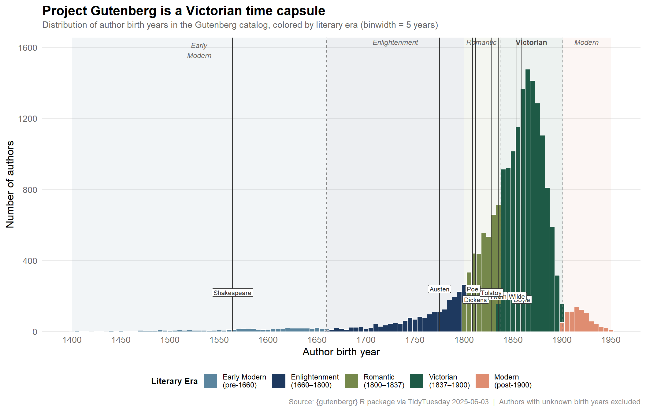
    title = "**Project Gutenberg is a Victorian time capsule**",
    subtitle = "Distribution of author birth years in the Gutenberg catalog, colored by literary era (binwidth = 5 years)",
    x = "Author birth year",
    y = "Number of authors",
    caption = "Source: {gutenbergr} R package via TidyTuesday 2025-06-03  |  Authors with unknown birth years excluded"
  ) +
  theme_minimal(base_size = 13) +
  theme(
    plot.title = element_markdown(face = "bold", size = 16, margin = margin(b = 4)),
    plot.subtitle = element_text(color = "gray40", size = 11, margin = margin(b = 10)),
    plot.caption = element_text(color = "gray55", size = 9),
    legend.position = "bottom",
    legend.title = element_text(size = 10, face = "bold"),
    legend.text = element_text(size = 9),
    panel.grid.minor = element_blank(),
    panel.grid.major.x = element_blank(),
    axis.text = element_text(color = "gray40")
  )

p_hero

ImportantThe Victorian Spike

The histogram reveals a pronounced spike centered around authors born between 1840 and 1880. This isn’t coincidence — it reflects Project Gutenberg’s copyright structure. Authors who died before 1928 (approximately) have works in the US public domain. Someone born in 1850 who lived 70 years died in 1920, well within that window. The Victorian era is therefore structurally over-represented in any public domain digital library.

How Prolific Were Gutenberg’s Most Represented Authors?

# Join metadata with authors to count works per author
works_per_author <- gutenberg_metadata %>%
  filter(!is.na(gutenberg_author_id), has_text == TRUE) %>%
  count(gutenberg_author_id, name = "n_works") %>%
  left_join(
    gutenberg_authors %>% select(gutenberg_author_id, author, birthdate, deathdate),
    by = "gutenberg_author_id"
  ) %>%
  filter(!is.na(author)) %>%
  arrange(desc(n_works))

cat(sprintf("works_per_author: %d rows\n", nrow(works_per_author)))
works_per_author: 25967 rows
stopifnot("works_per_author is empty" = nrow(works_per_author) > 0)

# Top 15 most represented authors
top_authors <- works_per_author %>%
  slice_head(n = 15) %>%
  mutate(
    # Clean author display name (last, first -> first last)
    author_display = str_replace(author, "^(.*?),\\s*(.*)$", "\\2 \\1"),
    author_display = fct_reorder(author_display, n_works),
    lifespan = ifelse(
      !is.na(birthdate) & !is.na(deathdate),
      paste0("(", birthdate, "–", deathdate, ")"),
      ""
    )
  )

cat("\nTop 10 most-represented authors:\n")

Top 10 most-represented authors:
top_authors %>%
  select(author_display, n_works, birthdate, deathdate) %>%
  head(10) %>%
  print()
# A tibble: 10 × 4
   author_display                     n_works birthdate deathdate
   <fct>                                <int>     <dbl>     <dbl>
 1 Various                               3961        NA        NA
 2 Anonymous                              929        NA        NA
 3 William Shakespeare                    334      1564      1616
 4 Mark Twain                             250      1835      1910
 5 Edward Bulwer Lytton, Baron Lytton     226      1803      1873
 6 Charles Dickens                        197      1812      1870
 7 Georg Ebers                            177      1837      1898
 8 Jules Verne                            176      1828      1905
 9 Alexandre Dumas                        165      1802      1870
10 Honoré de Balzac                       159      1799      1850
p_authors <- top_authors %>%
  ggplot(aes(x = n_works, y = author_display)) +
  geom_segment(
    aes(x = 0, xend = n_works, y = author_display, yend = author_display),
    color = as.character(era_palette[4]),
    linewidth = 0.9
  ) +
  geom_point(color = as.character(era_palette[1]), size = 4) +
  geom_text(
    aes(label = paste0(n_works, " works")),
    hjust = -0.2,
    size = 3.2,
    color = "gray30"
  ) +
  scale_x_continuous(expand = expansion(mult = c(0, 0.25))) +
  labs(
    title = "Prolific and public domain",
    subtitle = "Top 15 most-represented authors in Project Gutenberg by number of available text files",
    x = "Number of works with text",
    y = NULL,
    caption = "Source: {gutenbergr} R package via TidyTuesday 2025-06-03"
  ) +
  theme_minimal(base_size = 12) +
  theme(
    panel.grid.major.y = element_blank(),
    panel.grid.minor = element_blank(),
    plot.title = element_text(face = "bold", size = 14),
    plot.subtitle = element_text(color = "gray40", size = 10)
  )

p_authors


Update Palette Log

palette_log_path <- here::here("posts", "palette-log.csv")
palette_log <- read.csv(palette_log_path)

new_entry <- data.frame(
  post_date = "2025-06-03",
  palette   = "Redon",
  package   = "MetBrewer",
  type      = "discrete"
)

# Only append if this post_date + palette combo isn't already logged
if (!any(palette_log$post_date == new_entry$post_date &
         palette_log$palette   == new_entry$palette)) {
  write.table(
    new_entry,
    palette_log_path,
    append    = TRUE,
    sep       = ",",
    row.names = FALSE,
    col.names = FALSE
  )
  cat("Palette log updated: MetBrewer::Redon added for 2025-06-03\n")
} else {
  cat("Palette already logged — no duplicate written\n")
}

Final Thoughts and Takeaways

Project Gutenberg is the internet’s oldest digital library, and this dataset makes its character legible: it is overwhelmingly a Victorian archive, in English, dominated by fiction.

Three key findings:

  1. The temporal fingerprint is structural, not accidental. The spike of authors born between 1840–1880 is a direct consequence of US copyright law. Public domain status in the United States historically flipped at publication before 1928. Authors who flourished during the Victorian era fall squarely within this window. This means Gutenberg systematically over-represents the 19th century and under-represents the 20th.

  2. English is the dominant language by a massive margin. Even in the top-20, non-English languages represent a small fraction of the total. The collection’s founding context — North American and British digitization efforts of the early internet era — explains this. Finnish appearing high in the list is a genuine outlier worth exploring: sustained national investment in open cultural heritage digitization.

  3. Fiction, history, and poetry are the core subjects. The LCSH subjects confirm that Gutenberg is primarily a literary archive, not a scientific or technical one. “Science fiction” and “Detective and mystery stories” appearing in the top subjects reflects both the genre’s Victorian origins (Doyle, Verne, Wells) and Gutenberg’s cultural moment.

Limitation to note: Because we’re working with author metadata rather than publication records, this analysis measures who is in the collection, not when works were published or when they were digitized. A fuller picture would cross-reference publication dates and digitization timestamps.

The next time you reach for a Gutenberg text, you’re most likely picking up something an English-speaking Victorian novelist wrote between the Great Exhibition and the First World War. That’s not a flaw — it’s the shape of the public domain itself.