Tidy Tuesday: API Specs

tidytuesday

apis

web

technology

openapi

Mapping the web API ecosystem through APIs.guru’s catalog — who provides the most, what categories dominate, and how modern is the spec landscape?

Author

Sean Thimons

Published

June 17, 2025

Preface

From the TidyTuesday repository.

This week we’re exploring Web APIs! The dataset was curated by Jon Harmon while developing tools for creating API-wrapping R packages. The data comes from APIs.guru, whose goal is to create a “machine-readable Wikipedia for Web APIs in the OpenAPI Specification format.” Five tables cover API metadata, categories, logos, origin formats, and core specification details.

Loading necessary packages

My handy booster pack that allows me to install (if needed) and load my usual and favorite packages, as well as some helpful functions.

Code

# Packages ----------------------------------------------------------------

{
  # Install pak if it's not already installed
  if (!requireNamespace("pak", quietly = TRUE)) {
    install.packages(
      "pak",
      repos = sprintf(
        "https://r-lib.github.io/p/pak/stable/%s/%s/%s",
        .Platform$pkgType,
        R.Version()$os,
        R.Version()$arch
      )
    )
  }

  # CRAN Packages ----
  install_booster_pack <- function(package, load = TRUE) {
    for (pkg in package) {
      if (!requireNamespace(pkg, quietly = TRUE)) {
        pak::pkg_install(pkg)
      }
      if (load) {
        library(pkg, character.only = TRUE)
      }
    }
  }

  booster_pack <- c(
    ### IO ----
    'fs',
    'here',
    'janitor',
    'rio',
    'tidyverse',

    ### EDA ----
    'skimr',

    ### Plot ----
    'paletteer',           # Color palette collection
    'patchwork',           # Multi-panel layouts
    'ggtext',              # Rich text in ggplot
    'ggrepel',             # Non-overlapping labels

    ### Misc ----
    'tidytuesdayR'
  )

  install_booster_pack(package = booster_pack, load = TRUE)
  rm(install_booster_pack, booster_pack)

  # Custom Functions ----

  `%ni%` <- Negate(`%in%`)

  geometric_mean <- function(x) {
    exp(mean(log(x[x > 0]), na.rm = TRUE))
  }

  my_skim <- skim_with(
    numeric = sfl(
      n = length,
      min = ~ min(.x, na.rm = T),
      p25 = ~ stats::quantile(., probs = .25, na.rm = TRUE, names = FALSE),
      med = ~ median(.x, na.rm = T),
      p75 = ~ stats::quantile(., probs = .75, na.rm = TRUE, names = FALSE),
      max = ~ max(.x, na.rm = T),
      mean = ~ mean(.x, na.rm = T),
      geo_mean = ~ geometric_mean(.x),
      sd = ~ stats::sd(., na.rm = TRUE),
      hist = ~ inline_hist(., 5)
    ),
    append = FALSE
  )
}

Load raw data from package

raw <- tidytuesdayR::tt_load('2025-06-17')

apisguru_apis <- raw$apisguru_apis %>% janitor::clean_names()
api_categories <- raw$api_categories %>% janitor::clean_names()
api_info       <- raw$api_info       %>% janitor::clean_names()
api_logos      <- raw$api_logos      %>% janitor::clean_names()
api_origins    <- raw$api_origins    %>% janitor::clean_names()

Exploratory Data Analysis

The my_skim() function returns count, min, percentiles, mean, geometric mean, standard deviation, and an ASCII histogram.

`apisguru_apis` — the core catalog

This table has one row per API (filtered to the preferred version only), with timing metadata and spec version info. I drop swagger_url, link, external_docs_url, and external_docs_description since they are mostly URLs and free-text that won’t add to the numeric profile.

apisguru_apis %>%
  select(-swagger_url, -link, -external_docs_url, -external_docs_description) %>%
  my_skim()

Data summary
Name	Piped data
Number of rows	2529
Number of columns	5
_______________________
Column type frequency:
character	3
POSIXct	2
________________________
Group variables	None

Variable type: character

skim_variable	n_missing	complete_rate	min	max	n_unique
name	0	1	6	71	2529
version	1	1	1	43	643
openapi_ver	0	1	3	5	6

Variable type: POSIXct

skim_variable	n_missing	complete_rate	min	max	median	n_unique
added	0	1	2015-06-11 00:06:11	2023-04-20 23:20:25	2020-02-28 16:47:57	1113
updated	0	1	2016-04-10 23:18:20	2023-04-21 23:18:02	2021-02-07 16:23:46	524

`api_info` — provider, title, and license metadata

This table carries the richest semantic information. I drop free-text columns (description, contact_url, license_url, terms_of_service) that won’t contribute to the statistical profile, keeping the categorically interesting fields.

api_info %>%
  select(name, contact_name, title, provider_name, service_name,
         license_name) %>%
  my_skim()

Data summary
Name	Piped data
Number of rows	2529
Number of columns	6
_______________________
Column type frequency:
character	6
________________________
Group variables	None

Variable type: character

skim_variable	n_missing	complete_rate	min	max	n_unique	whitespace
name	0	1.00	6	71	2529	0
contact_name	1504	0.41	3	55	234	0
title	12	1.00	3	147	2050	0
provider_name	0	1.00	5	35	676	0
service_name	535	0.79	2	61	1934	0
license_name	1643	0.35	1	61	91	1

`api_categories` — many-to-many category assignments

cat(sprintf("api_categories: %d rows, %d cols\n",
            nrow(api_categories), ncol(api_categories)))

api_categories: 2783 rows, 2 cols

api_categories %>%
  count(apisguru_category, sort = TRUE) %>%
  head(20)

# A tibble: 20 × 2
   apisguru_category     n
   <chr>             <int>
 1 cloud               955
 2 media               340
 3 open_data           318
 4 analytics           284
 5 developer_tools     168
 6 ecommerce            78
 7 financial            72
 8 messaging            62
 9 entertainment        61
10 telecom              60
11 text                 57
12 location             51
13 collaboration        38
14 payment              32
15 transport            29
16 hosting              20
17 security             19
18 iot                  18
19 social               18
20 tools                16

`api_origins` — source spec formats

api_origins %>%
  count(format, sort = TRUE)

# A tibble: 7 × 2
  format           n
  <chr>        <int>
1 swagger       1060
2 openapi        923
3 <NA>           272
4 google         258
5 postman         15
6 wadl             5
7 apiBlueprint     3

The EDA reveals several things at a glance. The apisguru_apis catalog spans thousands of APIs with added dates spread over many years. The api_info table confirms that provider_name is the key grouping variable — providers supply anywhere from one to hundreds of services. Licenses are sparsely populated (many NAs), suggesting the API ecosystem is not yet mature in its licensing practices. In api_origins, swagger dominates as the original spec format, followed by openapi and google (Google Discovery).

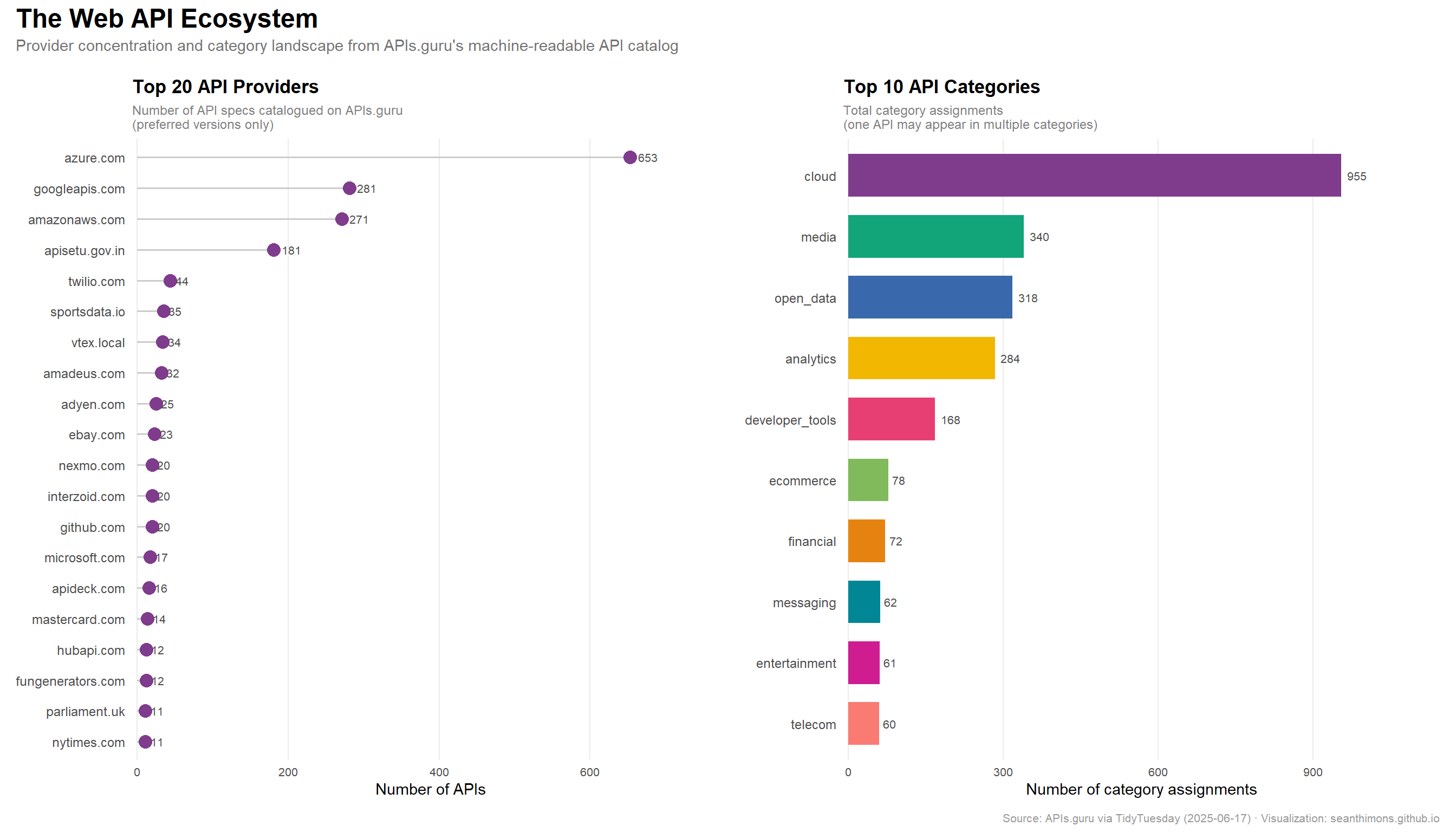
The Web API Ecosystem

Provider concentration: the long tail of API supply

How many APIs does each provider offer? The hypothesis is a classic power-law distribution: a handful of mega-providers (Amazon, Google, Microsoft) supply hundreds of APIs, while the vast majority of providers supply just one.

provider_counts <- api_info %>%
  filter(!is.na(provider_name)) %>%
  count(provider_name, sort = TRUE, name = "n_apis")

cat(sprintf("provider_counts: %d rows, %d cols\n",
            nrow(provider_counts), ncol(provider_counts)))

provider_counts: 676 rows, 2 cols

stopifnot("provider_counts is empty" = nrow(provider_counts) > 0)

# Distribution summary
provider_counts %>%
  summarise(
    total_providers = n(),
    single_api      = sum(n_apis == 1),
    pct_single      = round(100 * mean(n_apis == 1), 1),
    median_apis     = median(n_apis),
    max_apis        = max(n_apis),
    top_provider    = provider_name[which.max(n_apis)]
  )

# A tibble: 1 × 6
  total_providers single_api pct_single median_apis max_apis top_provider
            <int>      <int>      <dbl>       <dbl>    <int> <chr>       
1             676        599       88.6           1      653 azure.com

provider_counts %>% head(20)

# A tibble: 20 × 2
   provider_name     n_apis
   <chr>              <int>
 1 azure.com            653
 2 googleapis.com       281
 3 amazonaws.com        271
 4 apisetu.gov.in       181
 5 twilio.com            44
 6 sportsdata.io         35
 7 vtex.local            34
 8 amadeus.com           32
 9 adyen.com             25
10 ebay.com              23
11 github.com            20
12 interzoid.com         20
13 nexmo.com             20
14 microsoft.com         17
15 apideck.com           16
16 mastercard.com        14
17 fungenerators.com     12
18 hubapi.com            12
19 nytimes.com           11
20 parliament.uk         11

Note

The concentration is striking. The top provider alone offers tens to hundreds of API versions, while the majority of providers in the catalog contribute just a single spec. This is a textbook Pareto distribution — the “API ecosystem” looks like a busy marketplace only from the outside.

Category landscape

APIs.guru categorizes APIs with a many-to-many mapping — one API can belong to multiple categories. The counts below reflect total category assignments, not unique APIs.

category_counts <- api_categories %>%
  filter(!is.na(apisguru_category)) %>%
  count(apisguru_category, sort = TRUE, name = "n_apis")

cat(sprintf("category_counts: %d rows, %d cols\n",
            nrow(category_counts), ncol(category_counts)))

category_counts: 42 rows, 2 cols

stopifnot("category_counts is empty" = nrow(category_counts) > 0)

category_counts %>% head(20)

# A tibble: 20 × 2
   apisguru_category n_apis
   <chr>              <int>
 1 cloud                955
 2 media                340
 3 open_data            318
 4 analytics            284
 5 developer_tools      168
 6 ecommerce             78
 7 financial             72
 8 messaging             62
 9 entertainment         61
10 telecom               60
11 text                  57
12 location              51
13 collaboration         38
14 payment               32
15 transport             29
16 hosting               20
17 security              19
18 iot                   18
19 social                18
20 tools                 16

Licensing ecosystem

license_counts <- api_info %>%
  mutate(license_name = if_else(is.na(license_name), "(none / unlisted)", license_name)) %>%
  count(license_name, sort = TRUE, name = "n_apis")

license_counts %>% head(15)

# A tibble: 15 × 2
   license_name                                          n_apis
   <chr>                                                  <int>
 1 (none / unlisted)                                       1643
 2 Creative Commons Attribution 3.0                         285
 3 Apache 2.0 License                                       273
 4 Apache 2.0                                               109
 5 MIT                                                       51
 6 eBay API License Agreement                                25
 7 Interzoid license                                         20
 8 The MIT License (MIT)                                      7
 9 Open Government License - British Columbia                 6
10 U.S. Public Domain License                                 6
11 MIT License                                                4
12 open-licence                                               4
13 Apache-2.0                                                 3
14 BSD-3-Clause                                               3
15 API available under GNU Lesser General Public License      2

Important

The large proportion of APIs without a stated license reflects a recurring gap in the API ecosystem — many providers publish specs without explicit licensing terms, creating ambiguity for developers building on top of them.

Spec format: origin vs. APIs.guru’s served version

APIs.guru converts all ingested specs to OpenAPI format. This means an API originally written in Postman, WADL, or Google Discovery gets normalized and served in a common format. The api_origins table captures the original format, while apisguru_apis$openapi_ver reflects what APIs.guru actually serves.

# Original spec formats
origin_formats <- api_origins %>%
  filter(!is.na(format)) %>%
  count(format, sort = TRUE, name = "n_specs") %>%
  mutate(pct = round(100 * n_specs / sum(n_specs), 1))

cat("Origin formats:\n")

Origin formats:

print(origin_formats)

# A tibble: 6 × 3
  format       n_specs   pct
  <chr>          <int> <dbl>
1 swagger         1060  46.8
2 openapi          923  40.8
3 google           258  11.4
4 postman           15   0.7
5 wadl               5   0.2
6 apiBlueprint       3   0.1

# What APIs.guru serves (openapi version)
served_versions <- apisguru_apis %>%
  filter(!is.na(openapi_ver)) %>%
  mutate(
    major_ver = case_when(
      str_starts(openapi_ver, "3.1") ~ "OpenAPI 3.1.x",
      str_starts(openapi_ver, "3.0") ~ "OpenAPI 3.0.x",
      str_starts(openapi_ver, "2")   ~ "Swagger 2.0",
      TRUE                           ~ paste("Other:", openapi_ver)
    )
  ) %>%
  count(major_ver, sort = TRUE, name = "n_specs") %>%
  mutate(pct = round(100 * n_specs / sum(n_specs), 1))

cat("\nAPIs.guru served versions (grouped):\n")


APIs.guru served versions (grouped):

print(served_versions)

# A tibble: 3 × 3
  major_ver     n_specs   pct
  <chr>           <int> <dbl>
1 OpenAPI 3.0.x    1486  58.8
2 Swagger 2.0      1008  39.9
3 OpenAPI 3.1.x      35   1.4

Tip

Swagger → OpenAPI: The original format breakdown shows swagger-dominated origins, but APIs.guru also serves swagger 2.0 specs directly. The migration to OpenAPI 3.x is underway but not yet the majority — the ecosystem carries significant legacy.

Hero visualization: The Web API Ecosystem at a Glance

# --- palette --------------------------------------------------------------
# rcartocolor::Bold — 12 distinct colors, not previously used
cat_palette <- as.character(paletteer::paletteer_d("rcartocolor::Bold"))
provider_accent <- cat_palette[1]  # single accent for provider bars

# --- panel 1: top 20 providers -------------------------------------------
top20_providers <- provider_counts %>%
  head(20) %>%
  mutate(provider_name = fct_reorder(provider_name, n_apis))

cat(sprintf("top20_providers: %d rows\n", nrow(top20_providers)))

top20_providers: 20 rows

stopifnot("top20_providers is empty" = nrow(top20_providers) > 0)

p1 <- ggplot(top20_providers,
             aes(x = n_apis, y = provider_name)) +
  geom_segment(aes(x = 0, xend = n_apis,
                   y = provider_name, yend = provider_name),
               color = "grey80", linewidth = 0.6) +
  geom_point(size = 4, color = provider_accent) +
  geom_text(aes(label = n_apis),
            hjust = -0.4, size = 2.8, color = "grey30", family = "sans") +
  scale_x_continuous(expand = expansion(mult = c(0.01, 0.2))) +
  labs(
    title    = "Top 20 API Providers",
    subtitle = "Number of API specs catalogued on APIs.guru\n(preferred versions only)",
    x        = "Number of APIs",
    y        = NULL
  ) +
  theme_minimal(base_size = 11) +
  theme(
    plot.title       = element_text(face = "bold", size = 13),
    plot.subtitle    = element_text(color = "grey50", size = 9),
    panel.grid.major.y = element_blank(),
    panel.grid.minor   = element_blank(),
    axis.text.y      = element_text(size = 9),
    axis.text.x      = element_text(size = 8)
  )

# --- panel 2: top 10 categories ------------------------------------------
top10_cats <- category_counts %>%
  head(10) %>%
  mutate(
    apisguru_category = fct_reorder(apisguru_category, n_apis),
    fill_color        = cat_palette[seq_len(n())]
  )

cat(sprintf("top10_cats: %d rows\n", nrow(top10_cats)))

top10_cats: 10 rows

stopifnot("top10_cats is empty" = nrow(top10_cats) > 0)

p2 <- ggplot(top10_cats,
             aes(x = n_apis, y = apisguru_category, fill = apisguru_category)) +
  geom_col(width = 0.7, show.legend = FALSE) +
  geom_text(aes(label = n_apis),
            hjust = -0.3, size = 2.8, color = "grey30", family = "sans") +
  scale_fill_manual(values = setNames(top10_cats$fill_color,
                                      top10_cats$apisguru_category)) +
  scale_x_continuous(expand = expansion(mult = c(0.01, 0.2))) +
  labs(
    title    = "Top 10 API Categories",
    subtitle = "Total category assignments\n(one API may appear in multiple categories)",
    x        = "Number of category assignments",
    y        = NULL
  ) +
  theme_minimal(base_size = 11) +
  theme(
    plot.title       = element_text(face = "bold", size = 13),
    plot.subtitle    = element_text(color = "grey50", size = 9),
    panel.grid.major.y = element_blank(),
    panel.grid.minor   = element_blank(),
    axis.text.y      = element_text(size = 9),
    axis.text.x      = element_text(size = 8)
  )

# --- combine with patchwork ----------------------------------------------
p <- p1 + p2 +
  plot_annotation(
    title    = "The Web API Ecosystem",
    subtitle = "Provider concentration and category landscape from APIs.guru's machine-readable API catalog",
    caption  = "Source: APIs.guru via TidyTuesday (2025-06-17) · Visualization: seanthimons.github.io",
    theme    = theme(
      plot.title    = element_text(face = "bold", size = 18, margin = margin(b = 4)),
      plot.subtitle = element_text(color = "grey45", size = 11, margin = margin(b = 12)),
      plot.caption  = element_text(color = "grey60", size = 8, hjust = 1),
      plot.background = element_rect(fill = "white", color = NA)
    )
  )

p

Final thoughts and takeaways

The APIs.guru catalog is a snapshot of the public web API ecosystem in miniature — and it has the shape of almost every other technology ecosystem: power-law concentrated at the top, extraordinarily long-tailed below.

A single hyperscaler (Amazon Web Services, by most accounts) accounts for a disproportionate share of catalogued APIs. But this metric flatters the giants: one AWS region expanding its service surface area adds dozens of specs. The far more numerous single-API providers represent the quiet majority — independent developers, regional SaaS companies, and niche services that collectively outnumber the platform giants by a wide margin.

The category landscape confirms what the cloud era has wrought: “Cloud” and developer tooling dominate, followed by communication and IoT categories that reflect the proliferation of connected infrastructure. The long tail of the category chart captures verticals still in the early innings of API standardization.

The licensing gap is perhaps the most actionable finding. A large fraction of APIs in the catalog carry no stated license. For developers building client libraries or wrappers — exactly the use case Jon Harmon is addressing with his package ecosystem — that ambiguity matters. The rise of OpenAPI as a standardized spec format is one half of the interoperability story; clear licensing is the other half that the ecosystem hasn’t yet solved.

Finally, the spec format transition tells a gradualist story. Swagger 2.0 remains deeply embedded in the ecosystem’s origin history, but APIs.guru’s normalization layer and the slow uptick in OpenAPI 3.x adoption suggest the industry is moving — just not quickly.

Preface

Loading necessary packages

Load raw data from package

Exploratory Data Analysis

apisguru_apis — the core catalog

api_info — provider, title, and license metadata

api_categories — many-to-many category assignments

api_origins — source spec formats

The Web API Ecosystem

Provider concentration: the long tail of API supply

Category landscape

Licensing ecosystem

Spec format: origin vs. APIs.guru’s served version

Hero visualization: The Web API Ecosystem at a Glance

Final thoughts and takeaways

`apisguru_apis` — the core catalog

`api_info` — provider, title, and license metadata

`api_categories` — many-to-many category assignments

`api_origins` — source spec formats