Twenty-six years of British Library funding reveal a slow, sustained hollowing-out of government support — one that inflation makes far more dramatic than the nominal numbers suggest.
This dataset examines British Library funding trends from 1998–2023, compiled by Andy Jackson and inspired by David Rosenthal’s 2017 analysis documenting how “the inflation-adjusted income of the British Library fell between 1999 and 2016.” The data covers total reported funding broken into five streams — government grant-in-aid, voluntary contributions, investment returns, service delivery income, and other sources — alongside inflation adjustments to Year 2000 GBP.
Loading necessary packages
My handy booster pack that allows me to install (if needed) and load my usual and favorite packages, as well as some helpful functions.
raw <- tidytuesdayR::tt_load('2025-07-15')bl_funding <- raw$bl_funding %>% janitor::clean_names()
Exploratory Data Analysis
The my_skim() function is a modified version of the skimr::skim() function that returns the number of missing data points (cells as NA) as well as the inverse, the count, minimum, 25%, median, 75%, max, mean, geometric mean, and standard deviation. It also generates a little ASCII histogram. Neat!
bl_funding
# Drop free-text / redundant columns before skimmingbl_funding %>%select(-year_2000_gbp_millions) %>%# Rosenthal historical column — sparse overlapmy_skim()
Data summary
Name
Piped data
Number of rows
26
Number of columns
16
_______________________
Column type frequency:
numeric
16
________________________
Group variables
None
Variable type: numeric
skim_variable
n_missing
complete_rate
n
min
p25
med
p75
max
mean
geo_mean
sd
hist
year
0
1
26
1998.00
2004.25
2010.50
2016.75
2023.00
2010.50
2010.49
7.65
▇▇▇▇▇
nominal_gbp_millions
0
1
26
110.20
119.74
123.45
140.40
159.20
129.17
128.56
13.00
▆▇▂▅▂
gia_gbp_millions
0
1
26
78.47
90.21
96.00
106.27
127.80
98.08
97.43
11.61
▃▇▅▃▁
voluntary_gbp_millions
0
1
26
2.85
6.48
9.23
10.48
31.88
9.85
8.62
5.85
▇▇▂▁▁
investment_gbp_millions
0
1
26
0.08
0.43
0.65
0.97
3.00
0.87
0.66
0.68
▇▃▂▁▁
services_gbp_millions
0
1
26
7.58
14.12
18.76
24.45
31.05
19.45
18.36
6.38
▂▇▂▆▃
other_gbp_millions
0
1
26
0.00
0.00
0.00
0.29
13.34
0.91
1.96
2.68
▇▁▁▁▁
inflation_adjustment
0
1
26
979089.11
1058411.54
1257736.82
1412736.97
1818796.76
1268145.70
1249103.41
228337.65
▇▃▆▂▂
total_y2000_gbp_millions
0
1
26
81.64
85.83
109.61
118.62
144.77
104.40
102.92
17.99
▇▁▆▃▁
percentage_of_y2000_income
0
1
26
0.74
0.78
0.99
1.08
1.31
0.95
0.93
0.16
▇▁▆▃▁
gia_y2000_gbp_millions
0
1
26
64.12
69.73
79.18
86.00
94.57
78.60
78.00
9.87
▇▃▅▅▅
voluntary_y2000_gbp_millions
0
1
26
2.85
5.39
6.82
8.69
28.99
7.78
6.90
4.94
▇▃▁▁▁
investment_y2000_gbp_millions
0
1
26
0.05
0.37
0.48
0.81
1.73
0.71
0.53
0.53
▆▇▂▁▃
services_y2000_gbp_millions
0
1
26
5.07
10.00
14.94
23.12
31.71
16.60
14.70
7.90
▇▃▅▃▃
other_y2000_gbp_millions
0
1
26
0.00
0.00
0.00
0.19
10.38
0.70
1.41
2.08
▇▁▁▁▁
gia_as_percent_of_peak_gia
0
1
26
0.68
0.74
0.84
0.91
1.00
0.83
0.82
0.10
▇▃▅▅▅
# Verify actual year range and row countcat(sprintf("bl_funding: %d rows, %d cols\n", nrow(bl_funding), ncol(bl_funding)))
The dataset spans 26 annual report years (1998–2023, where year denotes the start of the financial year). The pre-computed percentage_of_y2000_income column shows total funding as a proportion of the year-2000 baseline — making the story immediately legible: the British Library has been steadily losing real purchasing power since roughly 2009. The gia_as_percent_of_peak_gia column tells an even starker story about government grant-in-aid specifically.
Note
What is Grant-in-Aid? Grant-in-Aid (GIA) is the UK government’s core annual subsidy to the British Library, channelled through the Department for Culture, Media and Sport (DCMS). It accounts for the majority of the Library’s income and funds basic operations — staffing, collections maintenance, digitisation, and public access.
Austerity in the Stacks
The headline finding from this dataset is not complex: government support for the British Library, once you strip away the fiction of nominal growth, has been cut persistently and deeply. But the composition story — how the funding mix has shifted as GIA has retreated — adds important texture.
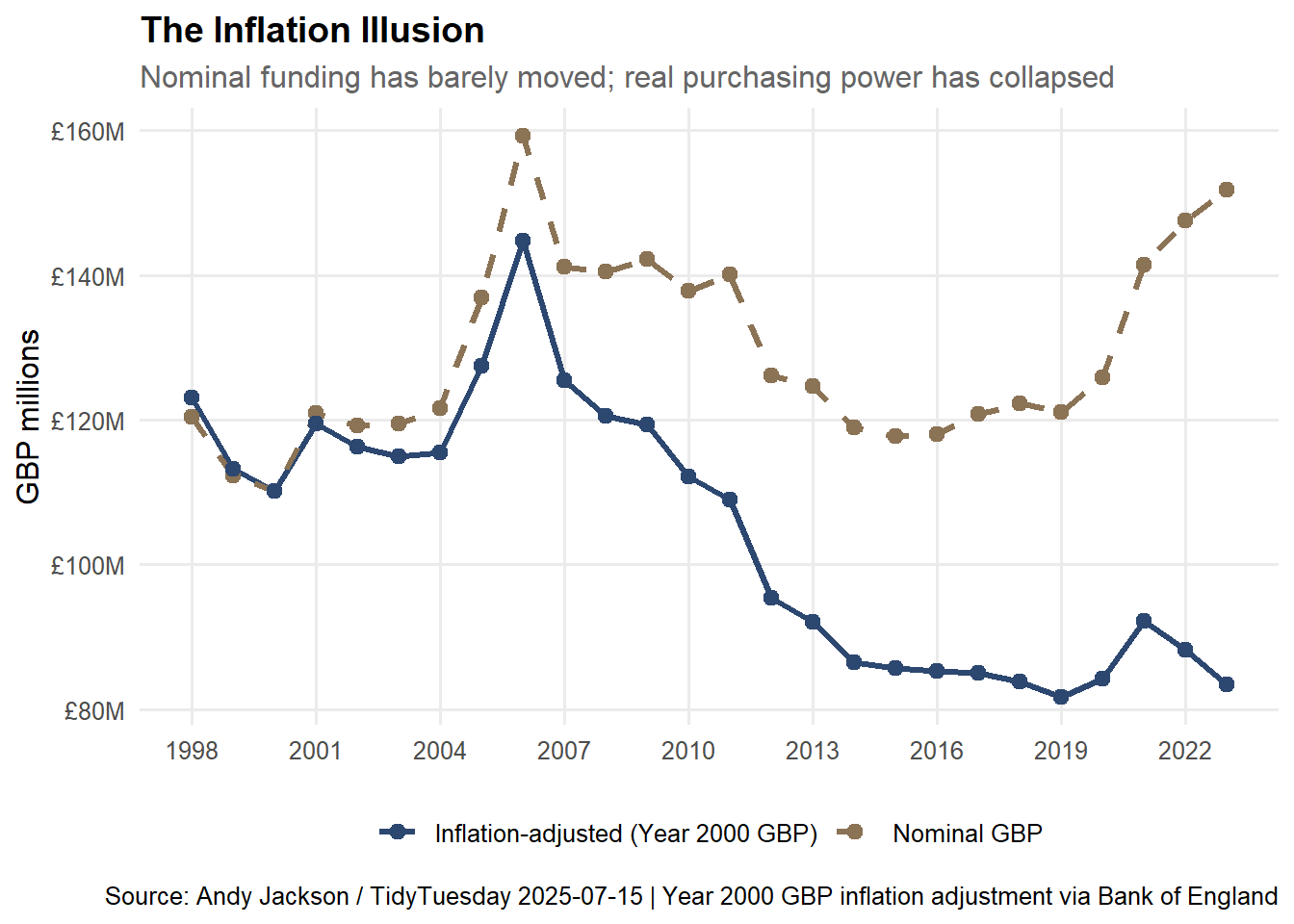
Nominal vs. Real: The Inflation Illusion
# Build a comparison of nominal vs. inflation-adjusted total fundingfunding_comparison <- bl_funding %>%select(year, nominal_gbp_millions, total_y2000_gbp_millions) %>%pivot_longer(cols =c(nominal_gbp_millions, total_y2000_gbp_millions),names_to ="measure",values_to ="gbp_millions" ) %>%mutate(measure =case_when( measure =="nominal_gbp_millions"~"Nominal GBP", measure =="total_y2000_gbp_millions"~"Inflation-adjusted (Year 2000 GBP)" ) )cat(sprintf("funding_comparison: %d rows, %d cols\n", nrow(funding_comparison), ncol(funding_comparison)))
funding_comparison: 52 rows, 3 cols
stopifnot("Plot data has 0 rows"=nrow(funding_comparison) >0)# Check both measures are presentstopifnot("Missing measure levels"=length(unique(funding_comparison$measure)) ==2)p_nominal <- ggplot2::ggplot( funding_comparison, ggplot2::aes(x = year, y = gbp_millions, color = measure, linetype = measure)) + ggplot2::geom_line(linewidth =1.2) + ggplot2::geom_point(size =2.5) + ggplot2::scale_color_manual(values =c("Nominal GBP"="#8B7355","Inflation-adjusted (Year 2000 GBP)"="#2C4770" ) ) + ggplot2::scale_linetype_manual(values =c("Nominal GBP"="dashed", "Inflation-adjusted (Year 2000 GBP)"="solid") ) + ggplot2::scale_y_continuous(labels = scales::label_dollar(prefix ="£", suffix ="M")) + ggplot2::scale_x_continuous(breaks =seq(1998, 2023, by =3)) + ggplot2::labs(title ="The Inflation Illusion",subtitle ="Nominal funding has barely moved; real purchasing power has collapsed",x =NULL,y ="GBP millions",color =NULL,linetype =NULL,caption ="Source: Andy Jackson / TidyTuesday 2025-07-15 | Year 2000 GBP inflation adjustment via Bank of England" ) + ggplot2::theme_minimal(base_size =12) + ggplot2::theme(legend.position ="bottom",plot.title = ggtext::element_markdown(face ="bold", size =14),plot.subtitle = ggtext::element_markdown(color ="grey40"),panel.grid.minor = ggplot2::element_blank() )p_nominal
The divergence between the two lines is the inflation illusion at work. Nominal funding appears roughly flat — even growing slightly after 2010. But once inflation is factored in, the British Library has been receiving steadily less real resource year after year.
stopifnot("gia_data is empty"=nrow(gia_data) >0)# Find peak GIA year for annotation# Column stored as proportion (0-1), not percentagepeak_gia_year <- gia_data %>%filter(gia_as_percent_of_peak_gia ==max(gia_as_percent_of_peak_gia, na.rm =TRUE)) %>%pull(year)cat(sprintf("Peak GIA year: %d\n", peak_gia_year))
Peak GIA year: 2007
# Most recent year's GIA as % of peak (multiply proportion by 100 for display)latest_gia_pct <- gia_data %>%filter(year ==max(year)) %>%pull(gia_as_percent_of_peak_gia) *100cat(sprintf("Latest GIA as %% of peak: %.1f%%\n", latest_gia_pct))
Latest GIA as % of peak: 74.3%
Important
GIA peaked in 2007 and by 2023 had fallen to 74% of that real peak. This is not a trivial fluctuation — it represents a sustained, decade-plus withdrawal of public investment in one of the country’s most important cultural institutions, driven by post-2008 austerity and successive DCMS budget cycles.
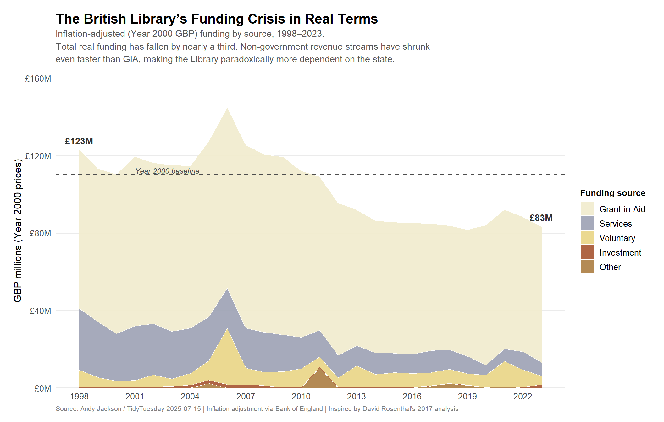
Funding Composition: The Stacked Story
To understand how the Library’s funding structure has evolved, we need to look at how the mix has shifted. The surprising finding: non-government revenue streams have not stepped in to compensate. They have collapsed in real terms even faster than GIA, making the Library paradoxically more dependent on government funding today than in 1998 — even as total resource has shrunk dramatically.
# Build annotation data for start and end totalstotals <- total_by_year %>%filter(year %in%c(min(year), max(year)))start_total <- totals %>%filter(year ==min(year)) %>%pull(total)end_total <- totals %>%filter(year ==max(year)) %>%pull(total)end_year <-max(total_by_year$year)start_year <-min(total_by_year$year)# Find the y position for end-of-series label (top of stack)label_data <- funding_long %>%group_by(year) %>%summarise(stack_top =sum(gbp_millions_y2000, na.rm =TRUE), .groups ="drop") %>%filter(year %in%c(start_year, end_year))p_hero <- ggplot2::ggplot( funding_long, ggplot2::aes(x = year, y = gbp_millions_y2000, fill = source)) + ggplot2::geom_area(alpha =0.92, color ="white", linewidth =0.3) +# Reference line: year 2000 baseline total ggplot2::geom_hline(yintercept =filter(total_by_year, year ==2000) %>%pull(total),linetype ="dashed",color ="grey30",linewidth =0.6 ) + ggplot2::annotate("text",x =2001,y =filter(total_by_year, year ==2000) %>%pull(total) +2,label ="Year 2000 baseline",color ="grey30",size =3.2,hjust =0,fontface ="italic" ) +# Start and end total callout labels ggrepel::geom_text_repel(data = label_data, ggplot2::aes(x = year,y = stack_top,label =sprintf("£%.0fM", stack_top) ),inherit.aes =FALSE,nudge_y =4,size =3.8,fontface ="bold",color ="grey20",segment.color ="grey50",segment.size =0.4,box.padding =0.4 ) + paletteer::scale_fill_paletteer_d("lisa::J_M_W_Turner") + ggplot2::scale_x_continuous(breaks =seq(1998, 2023, by =3)) + ggplot2::scale_y_continuous(labels = scales::label_dollar(prefix ="£", suffix ="M"),expand = ggplot2::expansion(mult =c(0, 0.12)) ) + ggplot2::labs(title ="**The British Library's Funding Crisis in Real Terms**",subtitle ="Inflation-adjusted (Year 2000 GBP) funding by source, 1998–2023.<br>Total real funding has fallen by nearly a third. Non-government revenue streams have shrunk<br>even faster than GIA, making the Library paradoxically more dependent on the state.",x =NULL,y ="GBP millions (Year 2000 prices)",fill ="Funding source",caption =paste0("Source: Andy Jackson / TidyTuesday 2025-07-15 | ","Inflation adjustment via Bank of England | ","Inspired by David Rosenthal's 2017 analysis" ) ) + ggplot2::theme_minimal(base_size =12) + ggplot2::theme(plot.title = ggtext::element_markdown(size =16, face ="bold", margin = ggplot2::margin(b =4)),plot.subtitle = ggtext::element_markdown(size =11, color ="grey35", lineheight =1.4, margin = ggplot2::margin(b =12)),plot.caption = ggplot2::element_text(size =8, color ="grey50", hjust =0),legend.position ="right",legend.title = ggplot2::element_text(face ="bold", size =10),legend.text = ggplot2::element_text(size =10),panel.grid.minor = ggplot2::element_blank(),panel.grid.major.x = ggplot2::element_blank(),axis.text = ggplot2::element_text(size =10),plot.margin = ggplot2::margin(16, 16, 12, 16) )p_hero
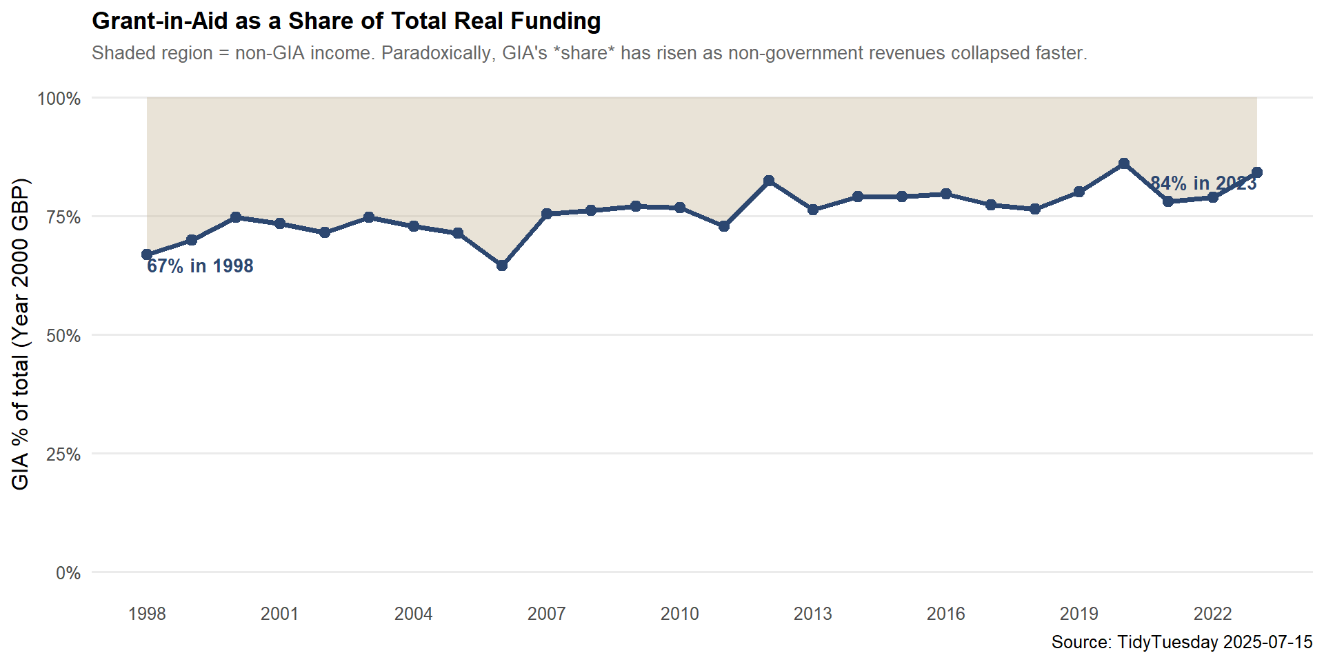
Supporting Analysis: GIA vs. Everything Else
# Compute GIA share of total real funding each yeargia_share <- bl_funding %>%transmute( year,gia_share = gia_y2000_gbp_millions / total_y2000_gbp_millions *100,other_share =100- gia_share )cat(sprintf("gia_share: %d rows\n", nrow(gia_share)))
# First and last year GIA share for annotationfirst_year <-min(gia_share$year)last_year <-max(gia_share$year)gia_first <- gia_share %>%filter(year == first_year) %>%pull(gia_share)gia_last <- gia_share %>%filter(year == last_year) %>%pull(gia_share)p_share <- ggplot2::ggplot(gia_share, ggplot2::aes(x = year, y = gia_share)) + ggplot2::geom_ribbon( ggplot2::aes(ymin = gia_share, ymax =100),fill ="#C8B89A", alpha =0.4 ) + ggplot2::geom_line(color ="#2C4770", linewidth =1.3) + ggplot2::geom_point(color ="#2C4770", size =2.5) + ggplot2::annotate("text",x = first_year, y = gia_first -2,label =sprintf("%.0f%% in %d", gia_first, first_year),hjust =0, size =3.5, color ="#2C4770", fontface ="bold" ) + ggplot2::annotate("text",x = last_year, y = gia_last -2,label =sprintf("%.0f%% in %d", gia_last, last_year),hjust =1, size =3.5, color ="#2C4770", fontface ="bold" ) + ggplot2::scale_y_continuous(limits =c(0, 100),labels = scales::label_percent(scale =1) ) + ggplot2::scale_x_continuous(breaks =seq(1998, 2023, by =3)) + ggplot2::labs(title ="Grant-in-Aid as a Share of Total Real Funding",subtitle ="Shaded region = non-GIA income. Paradoxically, GIA's *share* has risen as non-government revenues collapsed faster.",x =NULL,y ="GIA % of total (Year 2000 GBP)",caption ="Source: TidyTuesday 2025-07-15" ) + ggplot2::theme_minimal(base_size =12) + ggplot2::theme(plot.title = ggplot2::element_text(face ="bold", size =13),plot.subtitle = ggplot2::element_text(color ="grey40", size =10),panel.grid.minor = ggplot2::element_blank(),panel.grid.major.x = ggplot2::element_blank() )p_share
The share chart delivers a counterintuitive finding. GIA’s share of real total income has risen from around 67% in 1998 to 84% in 2023 — not because GIA has grown in real terms, but because everything else has fallen even faster. Services income, investment returns, and voluntary contributions have all contracted more steeply than GIA in inflation-adjusted terms. The Library is not diversifying away from government dependency; it is retreating toward it as the only source that has proved somewhat resilient.
Tip
What “services income” means here: Services income covers document supply, licensing, research partnerships, and paid access to specialist collections. In nominal terms this may have grown, but in real terms it has not kept pace with inflation — meaning the Library’s commercial activities are generating proportionally less purchasing power than they were 25 years ago.
Final thoughts and takeaways
Twenty-six years of British Library funding data tell a story that nominal figures deliberately obscure: the UK government has systematically reduced its real investment in one of the world’s great research libraries. In inflation-adjusted terms, the Library is operating on meaningfully less public resource than it was in the early 2000s, despite the dramatic expansion of its digital mandate and the rising cost of preserving born-digital collections.
A few takeaways worth holding onto:
The inflation illusion is real and consequential. Nominal GBP figures create a false impression of stability or even modest growth. Adjusting to Year 2000 prices reveals persistent, compounding decline — the kind that doesn’t announce itself in any single year but accumulates into structural underfunding over time.
Alternative income streams are insufficient substitutes. Services income, voluntary donations, and investment returns have all grown in real terms, but none has come close to compensating for the scale of GIA withdrawal. The Library is filling the gap through commercialisation and philanthropy, but these are inherently more volatile and mission-constrained revenue sources than core government grant.
This is an institutional resilience story as much as a funding story. The British Library has maintained world-class operations despite resource pressure, but that resilience has limits. Deferred digitisation, constrained collection growth, and reduced public programming are the hidden costs of austerity that don’t appear in a funding spreadsheet.
The data ends in 2023. The story, almost certainly, continues.