Through the Permanent Art Program, MTA Arts & Design (formerly Arts for Transit) commissions public art that is seen by millions of city-dwellers as well as national and international visitors who use the MTA’s subways and trains. Arts & Design works closely with the architects and engineers at MTA NYC Transit, Long Island Rail Road and Metro-North Railroad to determine the parameters and sites for the artwork that is to be incorporated into each station scheduled for renovation. A diversity of well-established, mid-career and emerging artists contribute to the growing collection of works created in the materials of the system — mosaic, ceramic, tile, bronze, steel and glass.
Dataset questions from TidyTuesday:
Which agency has the most art? Which has the least?
What are some common materials? How are details such as “hand forged” for bronze denoted in the data?
Loading necessary packages
My handy booster pack that allows me to install (if needed) and load my usual and favorite packages, as well as some helpful functions.
raw <- tidytuesdayR::tt_load('2025-07-22')mta_art <- raw$mta_artstation_lines <- raw$station_lines
Exploratory Data Analysis
The my_skim() function is a modified version of the skimr::skim() function that returns the number of missing data points (cells as NA) as well as the inverse (e.g.: number of rows that are notNA), the count, minimum, 25%, median, 75%, max, mean, geometric mean, and standard deviation. It also generates a little ASCII histogram. Neat!
mta_art
381 artworks commissioned by MTA agencies from 1980 through 2023. The art_image_link and line columns have minor missingness (5 and 3 NAs respectively). I’ll drop art_image_link and art_description from the skim — they’re free-text/URL fields that don’t profile usefully numerically.
The numeric column art_date (the installation year) spans 1980–2023, with a median of 2007 and a mean of 2007 — remarkably symmetric for a 43-year range. The ASCII histogram shows a right-leaning concentration in the 2000s and 2010s.
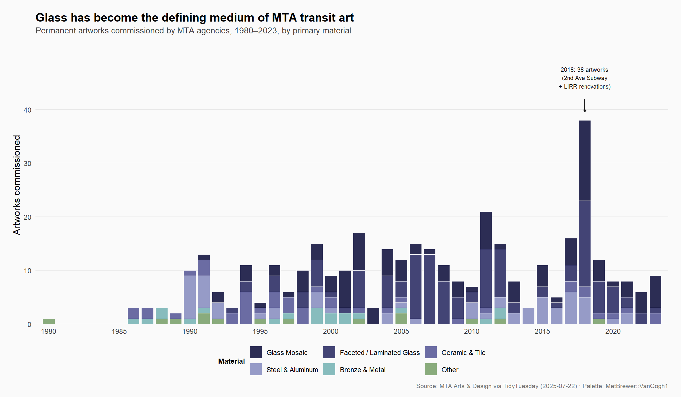
2018 stands out immediately — 38 artworks installed in a single year, nearly double the next-highest years. This warrants investigation.
station_lines
The companion dataset normalizes the line column from mta_art: each station-line pair gets its own row (720 rows for 381 artworks, since many stations serve multiple lines).
station_lines %>%my_skim()
Data summary
Name
Piped data
Number of rows
720
Number of columns
3
_______________________
Column type frequency:
character
3
________________________
Group variables
None
Variable type: character
skim_variable
n_missing
complete_rate
min
max
empty
n_unique
whitespace
agency
0
1
3
11
0
4
0
station_name
0
1
3
47
0
306
0
line
0
1
1
29
0
58
0
mta_art %>%count(agency, sort =TRUE)
# A tibble: 6 × 2
  agency              n
  <chr>           <int>
1 NYCT              293
2 Metro-North        43
3 LIRR               39
4 SIR                 3
5 MTA Bus Company     2
6 B&T                 1
NYCT (New York City Transit — the subway) accounts for 77% of all artworks. Metro-North (commuter rail north) and LIRR (Long Island Rail Road) are distant seconds at ~11% each. The Staten Island Railway (SIR) and MTA Bus Company are minor contributors.
The Material Language of Transit Art
The central creative constraint of the MTA Permanent Art Program is durability: artwork must survive decades of vibration, humidity, temperature swings, and 3+ million daily riders. The choice of material isn’t just aesthetic — it’s structural. Ceramic tile, mosaic, bronze, and glass aren’t choices made lightly.
NoteWhat’s “Faceted Glass”?
Faceted glass (also called dalle de verre) is a French technique using thick slabs of colored glass chipped to catch light at different angles — the same technique used in cathedral windows, adapted for transit stations. Laminated glass sandwiches colored elements between panes. Both are extremely durable and have dominated MTA commissions since the 1990s.
# Sanity check: verify no zero-row categoriesmat_counts <- art_classified %>%count(material_cat)stopifnot("All material categories must have > 0 rows"=all(mat_counts$n >0))cat(sprintf("art_classified: %d rows, %d cols — all material categories populated\n",nrow(art_classified), ncol(art_classified)))
art_classified: 381 rows, 10 cols — all material categories populated
Glass (mosaic + faceted/laminated) accounts for 61% of all 381 artworks. The next largest category — Steel & Aluminum — is a distant 13%.
# A tibble: 4 × 2
  agency          n
  <chr>       <int>
1 NYCT           25
2 LIRR           10
3 Metro-North     2
4 SIR             1
The 2018 spike is a multi-agency event, but the largest contributor is NYCT (23 artworks), followed by LIRR (10). This aligns with two concurrent capital programs:
ImportantThe 2018 Surge: Two Expansions at Once
Q Train Second Avenue Subway — Phase 1 opened January 1, 2017, adding three new stations (96 St, 86 St, 72 St) on the Upper East Side. Each station was designed from the ground up with permanent art commissions — a first for the MTA. The installations were completed and officially opened in 2017–2018.
LIRR / Metro-North Station Renovations — Several major Long Island and commuter rail stations received capital upgrades during this period, including Penn Station–area improvements and the Belmont Park area, each requiring new permanent art as part of ADA and structural renovation packages.
38 artworks in a single year is a record — about 3× the annual average over the prior decade.
Material Composition by Agency
agency_materials <- art_classified %>%filter(agency %in%c("NYCT", "Metro-North", "LIRR")) %>%count(agency, material_cat) %>%group_by(agency) %>%mutate(pct = n /sum(n)) %>%ungroup()cat("Material breakdown by agency:\n")
Metro-North’s collection leans more heavily on Steel & Aluminum (33% vs. 11% for NYCT) — a reflection of its newer station architecture, which favors industrial materials over mosaic traditions. NYCT’s long renovation history and the influence of the Arts for Transit program from the 1980s onward embedded glass mosaic as the canonical medium.
Hero Visualization: Four Decades of Material in Motion
# Check used palettespalette_log_path <- here::here("posts", "palette-log.csv")palette_log <-read.csv(palette_log_path)cat("Previously used palettes:\n")
# MetBrewer::VanGogh1 — 7 colors, artistic feel, not previously used# Perfect for 7 material categories in an art-themed datasetpaletteer::paletteer_d("MetBrewer::VanGogh1")
# Join art with station_lines to get per-line art countsart_by_line <- station_lines %>%inner_join( mta_art %>%select(agency, station_name, art_title),by =c("agency", "station_name"),relationship ="many-to-many" ) %>%# Only NYCT subway letter/number lines (exclude commuter rail names)filter(agency =="NYCT") %>%filter(nchar(line) <=2) %>%distinct(line, art_title) %>%count(line, sort =TRUE) %>%head(15)cat(sprintf("art_by_line: %d rows\n", nrow(art_by_line)))
art_by_line: 15 rows
stopifnot("art_by_line must not be empty"=nrow(art_by_line) >0)print(art_by_line)
# A tibble: 15 × 2
line n
<chr> <int>
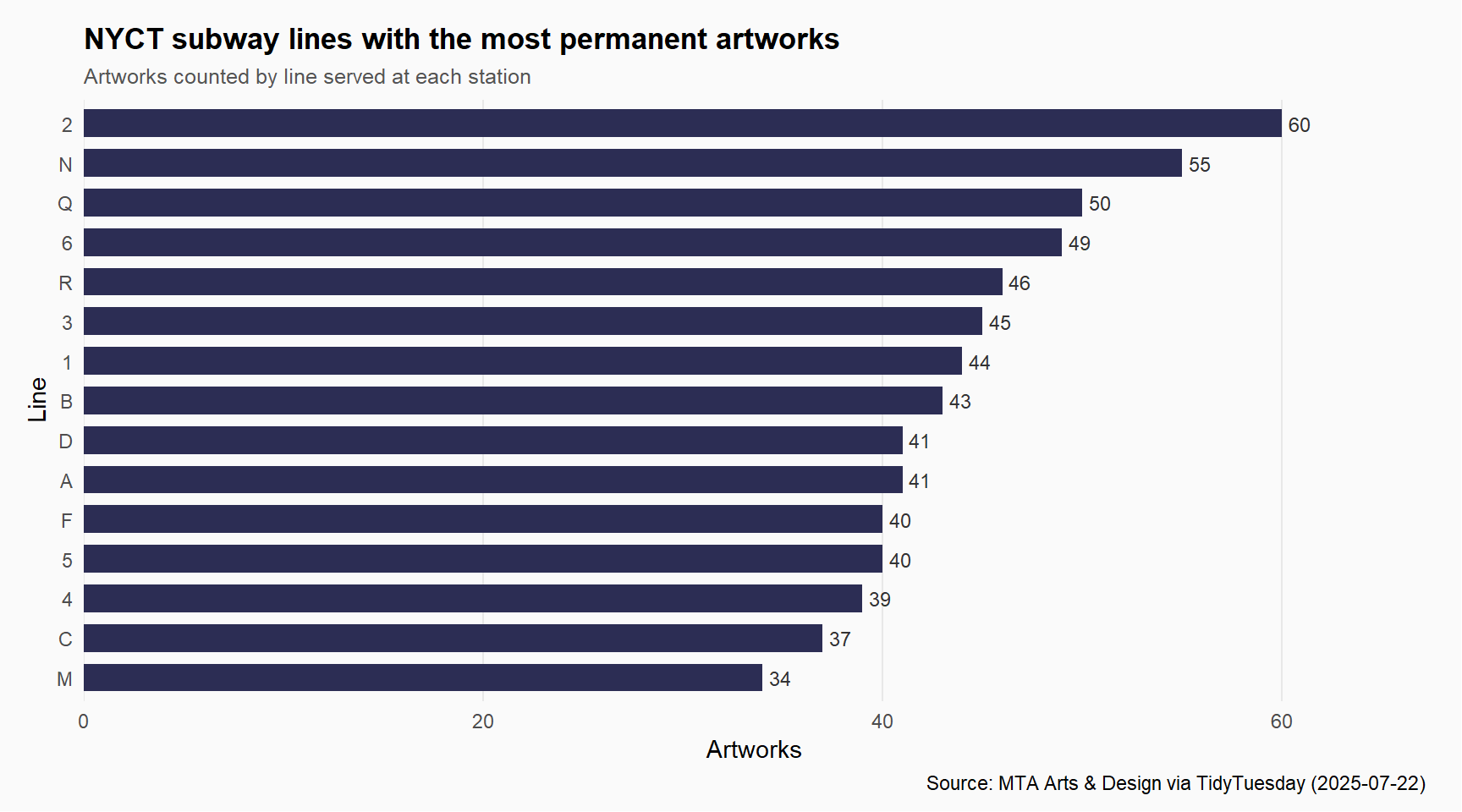
1 2 60
2 N 55
3 Q 50
4 6 49
5 R 46
6 3 45
7 1 44
8 B 43
9 A 41
10 D 41
11 5 40
12 F 40
13 4 39
14 C 37
15 M 34
line_order <- art_by_line %>%arrange(n) %>%pull(line)p2 <- art_by_line %>%mutate(line =factor(line, levels = line_order)) %>% ggplot2::ggplot(ggplot2::aes(x = n, y = line)) + ggplot2::geom_col(fill =unname(mat_colors["Glass Mosaic"]), width =0.7) + ggplot2::geom_text( ggplot2::aes(label = n),hjust =-0.3,size =3.2,color ="#333333" ) + ggplot2::scale_x_continuous(expand = ggplot2::expansion(mult =c(0, 0.12)) ) + ggplot2::labs(title ="NYCT subway lines with the most permanent artworks",subtitle ="Artworks counted by line served at each station",x ="Artworks",y ="Line",caption ="Source: MTA Arts & Design via TidyTuesday (2025-07-22)" ) + ggplot2::theme_minimal(base_size =11) + ggplot2::theme(plot.title = ggplot2::element_text(face ="bold", size =13),plot.subtitle = ggplot2::element_text(color ="#555555", size =9.5),panel.grid.major.y = ggplot2::element_blank(),panel.grid.minor = ggplot2::element_blank(),panel.grid.major.x = ggplot2::element_line(color ="#e8e8e8"),plot.margin = ggplot2::margin(12, 16, 8, 12),plot.background = ggplot2::element_rect(fill ="#fafafa", color =NA) )p2
The 2, 3, 4, 5, 6 IRT lines (the original numbered subway trunks through Manhattan) dominate, reflecting both their age and the MTA’s longstanding renovation cycles. The Q line ranks highly due to the Second Avenue Subway stations — each of which received purpose-built, high-profile commissions.
Final thoughts and takeaways
Four decades of the MTA Permanent Art Catalog tell a clear story: glass won. What began as a program grounded in traditional transit materials — bronze plaques, ceramic tile, terrazzo floors — transformed into a nearly glass-exclusive medium by the 2010s.
This isn’t just aesthetic preference. Glass mosaic and faceted glass survive underground environments exceptionally well: they’re impervious to moisture, easy to clean, and unlike paint or fiber, they don’t fade under fluorescent light. The MTA’s experience over decades of maintenance reinforced glass as the practical and artistic medium of choice.
The 2018 peak (38 artworks) is the catalog’s most dramatic signal: a confluence of the Second Avenue Subway Q train opening and concurrent LIRR/Metro-North capital programs created a one-time windfall for public art commissioning. Those three Second Avenue stations — 96 St, 86 St, and 72 St — represent some of the most ambitious transit art installations in American history, with commissions from Chuck Close, Vik Muniz, and Jean Shin.
A few caveats worth noting:
Material classification is imprecise. The art_material column is free text with significant inconsistency ("Faceted glass", "faceted glass", "Faceted Glass" are all present). My classification captures the spirit, not every edge case.
Dates reflect installation, not commission. The bureaucratic lag between commissioning and installation means the 2018 artworks were likely contracted 3–5 years earlier.
The catalog is incomplete at the margins. Some early artworks (1980–1985) may be underdocumented, and the most recent years likely have works in progress not yet captured.
The MTA’s underground gallery is one of New York City’s most-visited — and least-considered — art collections. 381 permanent works. Millions of daily viewers who mostly stare at their phones.