Tidy Tuesday: What Have We Been Watching on Netflix?
tidytuesday
R
netflix
entertainment
streaming
Analyzing Netflix’s engagement reports from H2 2023 through H1 2025 to reveal what titles dominated global viewing—and why international content is quietly running the platform.
Netflix publishes semi-annual “What We Watched” engagement reports covering approximately 99% of all viewing activity. This dataset compiles four consecutive reports—H2 2023, H1 2024, H2 2024, and H1 2025—spanning both movies and TV shows, with total hours viewed, runtime, implied view counts, and global availability status for each title.
Suggested questions from the dataset:
How do older titles compare to newer releases in sustained viewership?
Does release timing (month/season) influence engagement?
Are globally available titles more popular than regionally restricted ones?
Which movie types consistently perform well across reporting periods?
How do later seasons of shows perform relative to earlier seasons?
Loading necessary packages
My handy booster pack that allows me to install (if needed) and load my usual and favorite packages, as well as some helpful functions.
The my_skim() function is a modified version of the skimr::skim() function that returns the number of missing data points (cells as NA) as well as the inverse (e.g.: number of rows that are notNA), the count, minimum, 25%, median, 75%, max, mean, geometric mean, and standard deviation. It also generates a little ASCII histogram. Neat!
Movies
# Drop source (redundant with report) and runtime (character, parsed separately)movies %>%select(-source, -runtime) %>%my_skim()
Data summary
Name
Piped data
Number of rows
36121
Number of columns
7
_______________________
Column type frequency:
character
4
Date
1
numeric
2
________________________
Group variables
None
Variable type: character
skim_variable
n_missing
complete_rate
min
max
empty
n_unique
whitespace
report
0
1
11
11
0
4
0
title
6
1
1
144
0
13551
0
available_globally
9
1
2
19
0
3
0
content_type
0
1
5
5
0
1
0
Variable type: Date
skim_variable
n_missing
complete_rate
min
max
median
n_unique
release_date
29396
0.19
2013-12-12
2025-06-30
2021-08-13
1128
Variable type: numeric
skim_variable
n_missing
complete_rate
n
min
p25
med
p75
max
mean
geo_mean
sd
hist
hours_viewed
12
1
36121
1e+05
2e+05
4e+05
1900000
313000000
2790858
606805.6
9054284
▇▁▁▁▁
views
12
1
36121
1e+05
1e+05
3e+05
1100000
164700000
1573256
392923.0
4974895
▇▁▁▁▁
The movies dataset spans 36,121 entries across four semi-annual reporting periods. The median movie earned around 400,000 hours of viewing—which sounds impressive until you notice the mean is nearly 7× higher at 2.8M hours, signaling a heavily right-skewed distribution. A small number of blockbusters are dragging the mean far above the typical title. Release date is missing for roughly 80% of entries, so temporal analysis will be limited to the report period rather than individual release dates.
Shows
shows %>%select(-source, -runtime) %>%my_skim()
Data summary
Name
Piped data
Number of rows
27803
Number of columns
7
_______________________
Column type frequency:
character
4
Date
1
numeric
2
________________________
Group variables
None
Variable type: character
skim_variable
n_missing
complete_rate
min
max
empty
n_unique
whitespace
report
0
1
11
11
0
4
0
title
6
1
3
225
0
9913
0
available_globally
9
1
2
19
0
3
0
content_type
0
1
4
4
0
1
0
Variable type: Date
skim_variable
n_missing
complete_rate
min
max
median
n_unique
release_date
14033
0.5
2010-04-01
2025-06-30
2021-04-14
1968
Variable type: numeric
skim_variable
n_missing
complete_rate
n
min
p25
med
p75
max
mean
geo_mean
sd
hist
hours_viewed
12
1
27803
1e+05
8e+05
2500000
8200000
840300000
9807243
2621429.5
26327450
▇▁▁▁▁
views
12
1
27803
1e+05
2e+05
400000
1300000
144800000
1414994
497184.2
3665090
▇▁▁▁▁
TV shows tell a different story. With 27,803 entries, the catalog is smaller—but the numbers are much bigger. The median show earns 2.5M hours (6× a median movie), and the mean climbs to 9.8M hours. The top show in any single period earned 840M hours. Shows are also the “stickier” content: binge-watching entire seasons naturally accumulates more total hours than any single film.
Note
The available_globally column contains three artifact rows with the literal value "Available Globally?" (likely header rows from the original Excel export). These are filtered out during analysis.
The Netflix Viewing Landscape
# Combine, filter artifacts and missing hour datanetflix <-bind_rows(movies, shows) %>%filter(available_globally %in%c("Yes", "No")) %>%filter(!is.na(hours_viewed))# Flag international content: bilingual titles use " // " separator (mostly Korean)# Flag limited series: explicit format name in titlenetflix <- netflix %>%mutate(is_international =str_detect(title, " // "),is_limited_series =str_detect(title, "Limited Series"),title_display =if_else( is_international,str_remove(title, " //.*"), title ) )cat(sprintf("Combined clean dataset: %d rows, %d cols\n", nrow(netflix), ncol(netflix)))cat(sprintf("Movies: %d rows | Shows: %d rows\n",sum(netflix$content_type =="Movie"),sum(netflix$content_type =="Show")))
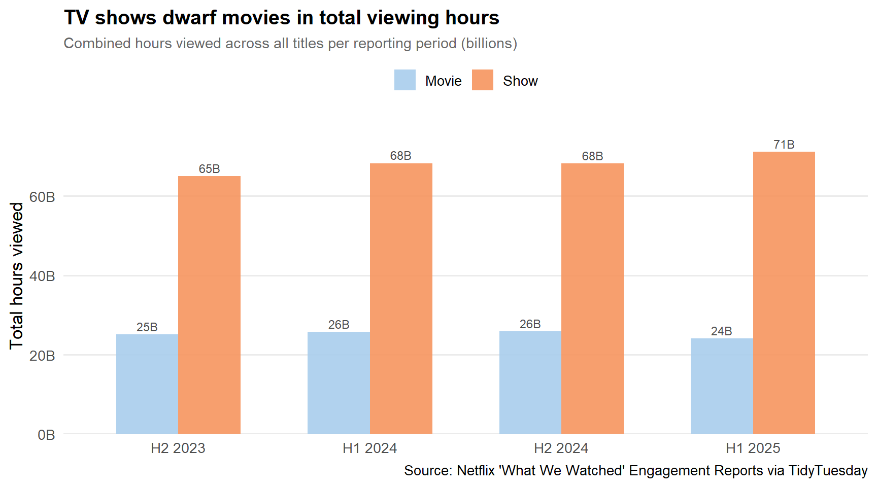
stopifnot("type_by_period has 0 rows"=nrow(type_by_period) >0)p_type <- type_by_period %>%ggplot(ggplot2::aes(x = report, y = total_hours_B, fill = content_type, group = content_type)) + ggplot2::geom_col(position ="dodge", width =0.65, alpha =0.9) + ggplot2::geom_text( ggplot2::aes(label =sprintf("%.0fB", total_hours_B)),position =position_dodge(width =0.65),vjust =-0.4, size =3.2, color ="grey30" ) + paletteer::scale_fill_paletteer_d("nationalparkcolors::Arches") + ggplot2::scale_y_continuous(labels = scales::label_number(suffix ="B"),expand = ggplot2::expansion(mult =c(0, 0.12)) ) + ggplot2::labs(title ="TV shows dwarf movies in total viewing hours",subtitle ="Combined hours viewed across all titles per reporting period (billions)",x =NULL,y ="Total hours viewed",fill =NULL,caption ="Source: Netflix 'What We Watched' Engagement Reports via TidyTuesday" ) + ggplot2::theme_minimal(base_size =13) + ggplot2::theme(legend.position ="top",plot.title = ggplot2::element_text(face ="bold", size =15),plot.subtitle = ggplot2::element_text(color ="grey40", size =11),panel.grid.major.x = ggplot2::element_blank(),panel.grid.minor = ggplot2::element_blank() )p_type
Across every reporting period, TV shows generate 3–4× more total hours than movies, despite having a smaller catalog. This isn’t simply a runtime effect—the views column (hours ÷ runtime) tells the same story. People return to shows, finish seasons, and re-watch episodes. Movies, for all their cultural prestige, are inherently one-and-done.
International Content’s Quiet Dominance
Netflix’s bilingual title convention—“Squid Game: Season 2 // 오징어 게임: 시즌 2”—makes international content easy to identify. These double-named titles are predominantly Korean dramas, though Spanish, Thai, and other language productions also use this format.
# A tibble: 4 × 6
  content_type is_international n_titles total_hours_B median_hours_M
  <chr>        <lgl>               <int>         <dbl>          <dbl>
1 Movie        FALSE               23252          83.8            0.7
2 Movie        TRUE                12857          17.0            0.3
3 Show         FALSE               18166         194.             2.9
4 Show         TRUE                 9625          78.8            2
# ℹ 1 more variable: language_label <chr>
Important
International shows—identifiable by their bilingual title format—account for a disproportionately large share of top viewership relative to their catalog size. Among shows in the top 25 all-time by total hours, roughly half carry a bilingual title.
Netflix’s Most-Watched Shows, H2 2023–H1 2025
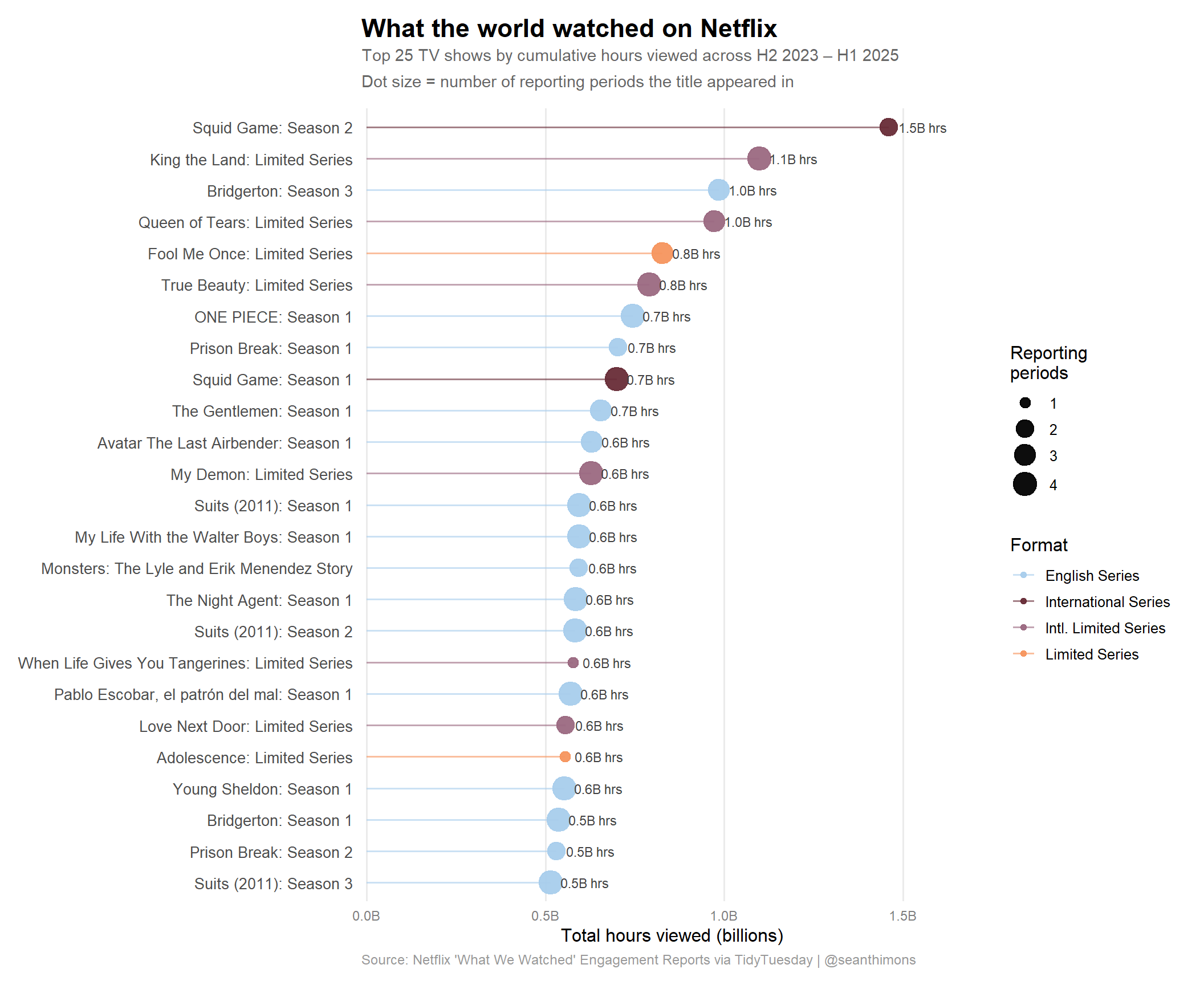
The central question: after aggregating all four reporting periods, which shows have racked up the most cumulative viewing time?
# Aggregate shows across all periods they appear intop_shows <- netflix %>%filter(content_type =="Show") %>%group_by(title, title_display, is_international, is_limited_series) %>%summarise(total_hours =sum(hours_viewed, na.rm =TRUE),n_periods =n_distinct(report),peak_hours =max(hours_viewed, na.rm =TRUE),.groups ="drop" ) %>%slice_max(total_hours, n =25) %>%mutate(hours_B = total_hours /1e9,content_label =case_when( is_international & is_limited_series ~"Intl. Limited Series", is_international ~"International Series", is_limited_series ~"Limited Series",TRUE~"English Series" ) )cat(sprintf("top_shows: %d rows\n", nrow(top_shows)))stopifnot("top_shows is empty"=nrow(top_shows) >0)# Verify we have variation in content_labelcat("Content label distribution:\n")print(table(top_shows$content_label))
# Select 4 colors from the Arches palette for 4 content label categoriesarch_colors <-as.character(paletteer::paletteer_d("nationalparkcolors::Arches"))# Map colors to content categories (Arches has 6 colors: light blue, orange, dark red, mauve, slate, warm gray)content_colors <-c("English Series"= arch_colors[1],"Limited Series"= arch_colors[2],"International Series"= arch_colors[3],"Intl. Limited Series"= arch_colors[4])# If any category isn't present, this won't break — scale_color_manual handles missing levelsp_hero <- top_shows %>%mutate(title_display =fct_reorder(title_display, hours_B),label_text =sprintf("%.1fB hrs", hours_B) ) %>% ggplot2::ggplot(ggplot2::aes(x = hours_B, y = title_display, color = content_label)) +# Segment from 0 to dot ggplot2::geom_segment( ggplot2::aes(x =0, xend = hours_B, yend = title_display),linewidth =0.7, alpha =0.6 ) +# Point sized by number of reporting periods ggplot2::geom_point(ggplot2::aes(size = n_periods), alpha =0.95) +# Hours label ggplot2::geom_text( ggplot2::aes(label = label_text),hjust =-0.2, size =3, color ="grey25" ) + ggplot2::scale_color_manual(values = content_colors,name ="Format" ) + ggplot2::scale_size_continuous(name ="Reporting\nperiods",range =c(3, 7),breaks =c(1, 2, 3, 4) ) + ggplot2::scale_x_continuous(labels = scales::label_number(suffix ="B"),expand = ggplot2::expansion(mult =c(0.01, 0.18)) ) + ggplot2::labs(title ="What the world watched on Netflix",subtitle ="Top 25 TV shows by cumulative hours viewed across H2 2023 – H1 2025\nDot size = number of reporting periods the title appeared in",x ="Total hours viewed (billions)",y =NULL,caption ="Source: Netflix 'What We Watched' Engagement Reports via TidyTuesday | @seanthimons" ) + ggplot2::theme_minimal(base_size =12) + ggplot2::theme(plot.title = ggplot2::element_text(face ="bold", size =17, margin = ggplot2::margin(b =4)),plot.subtitle = ggplot2::element_text(color ="grey40", size =11, lineheight =1.3,margin = ggplot2::margin(b =12)),plot.caption = ggplot2::element_text(color ="grey60", size =9, hjust =0),axis.text.y = ggplot2::element_text(size =10),axis.text.x = ggplot2::element_text(size =9, color ="grey50"),panel.grid.major.y = ggplot2::element_blank(),panel.grid.minor = ggplot2::element_blank(),panel.grid.major.x = ggplot2::element_line(color ="grey92"),legend.position ="right",legend.box ="vertical",plot.margin = ggplot2::margin(12, 16, 12, 12) )p_hero
A few things stand out immediately:
Squid Game is in a class of its own. Season 2 alone has accumulated well over a billion cumulative hours across two reporting periods—an almost incomprehensible figure. The franchise’s third season also debuted in the top tier within a single period.
Korean dramas dominate the top 10. “Bridgerton” and a handful of English-language limited series represent the American entries, but Queen of Tears, King the Land, and When Life Gives You Tangerines all rank among the most-watched titles globally. These are not niche imports—they are mainstream Netflix hits.
The “Limited Series” format is winning. Adolescence (4 episodes, British), Fool Me Once, Zero Day, and Monster are all limited series that outperformed most ongoing scripted shows. The format offers a complete, bingeable arc that maps perfectly onto how people actually consume streaming content.
Bigger dots = staying power. Titles appearing in multiple periods (the larger dots) are generally in the upper half of the chart, suggesting that sustained viewership compounds—a show that was big in H2 2024 often continued accumulating hours in H1 2025.
Final thoughts and takeaways
Netflix’s “What We Watched” data is a rare window into global media consumption at scale—and it tells a clear story.
TV shows are the engine of engagement. Movies attract cultural conversation and awards attention, but it’s serialized television that keeps people logged in. The gap in total hours—roughly 3–4× more for shows each period—is structural, not incidental.
The global content bet has paid off. When Netflix invested heavily in Korean, Spanish, and other non-English productions, skeptics worried that local content wouldn’t travel. The data says otherwise. Korean dramas now compete directly with Netflix’s English-language originals for the top of the global rankings, and in many periods they win outright.
“Limited Series” is the format of the moment. The binge-completion dynamic is maximized when a show has a defined ending. Adolescence—a 4-episode British drama—accumulated over half a billion hours despite its brevity. That’s the power of a show where people tell their friends “you have to finish it this weekend.”
The long tail is very long. The median movie earns around 400,000 hours in a reporting period. The top movie earns 313M hours. That’s a 783× difference. Netflix’s catalog strategy—keeping vast amounts of content available—means most titles are filler for the algorithm, present to serve niche moments while a handful of tentpoles do the heavy lifting.
One important caveat: this data only covers titles Netflix chooses to report. The engagement reports explicitly cover “~99% of all viewing,” but the threshold for inclusion (100,000+ hours in a period) still means many niche titles are invisible. The long tail is even longer than it appears here.