Tidy Tuesday: Australian Frogs

tidytuesday
R
ecology
citizen-science
australia
wildlife
Mapping the seasonal calling calendar of Australia’s frogs using 136,000 citizen-science observations from the 2023 FrogID survey.
Author

Sean Thimons

Published

September 2, 2025

Preface

From the TidyTuesday repository.

FrogID is a citizen science initiative allowing Australians to record and submit frog calls for expert identification. The 2023 dataset represents the sixth annual data release, contributing to over 30 scientific papers on frog ecology, taxonomy, and conservation since 2017. Australia hosts 257 native frog species found nowhere else on Earth — yet almost one in five species are threatened with extinction due to climate change, urbanisation, disease, and invasive species.

Suggested research questions:

  • Which frog species are endemic to specific Australian regions?
  • Do different species exhibit distinct seasonal calling patterns?
  • Which species has the broadest geographic distribution versus the most limited range?

Loading necessary packages

My handy booster pack that allows me to install (if needed) and load my usual and favorite packages, as well as some helpful functions.

Code
# Packages ----------------------------------------------------------------

{
  # Install pak if it's not already installed
  if (!requireNamespace("pak", quietly = TRUE)) {
    install.packages(
      "pak",
      repos = sprintf(
        "https://r-lib.github.io/p/pak/stable/%s/%s/%s",
        .Platform$pkgType,
        R.Version()$os,
        R.Version()$arch
      )
    )
  }

  # CRAN Packages ----
  install_booster_pack <- function(package, load = TRUE) {
    for (pkg in package) {
      if (!requireNamespace(pkg, quietly = TRUE)) {
        pak::pkg_install(pkg)
      }
      if (load) {
        library(pkg, character.only = TRUE)
      }
    }
  }

  booster_pack <- c(
    ### IO ----
    'fs',
    'here',
    'janitor',
    'rio',
    'tidyverse',

    ### EDA ----
    'skimr',

    ### Plot ----
    'paletteer',           # Color palette collection
    'ggtext',              # Rich text (italic species names)
    'ggrepel',             # Non-overlapping labels
    'scales',              # Axis formatting

    ### Misc ----
    'tidytuesdayR'
  )

  install_booster_pack(package = booster_pack, load = TRUE)
  rm(install_booster_pack, booster_pack)

  # Custom Functions ----

  `%ni%` <- Negate(`%in%`)

  geometric_mean <- function(x) {
    exp(mean(log(x[x > 0]), na.rm = TRUE))
  }

  my_skim <- skim_with(
    numeric = sfl(
      n = length,
      min = ~ min(.x, na.rm = T),
      p25 = ~ stats::quantile(., probs = .25, na.rm = TRUE, names = FALSE),
      med = ~ median(.x, na.rm = T),
      p75 = ~ stats::quantile(., probs = .75, na.rm = TRUE, names = FALSE),
      max = ~ max(.x, na.rm = T),
      mean = ~ mean(.x, na.rm = T),
      geo_mean = ~ geometric_mean(.x),
      sd = ~ stats::sd(., na.rm = TRUE),
      hist = ~ inline_hist(., 5)
    ),
    append = FALSE
  )
}

Load raw data from package

raw <- tidytuesdayR::tt_load('2025-09-02')

frog_data  <- raw$frogID_data   # 136,621 citizen-science observation records
frog_names <- raw$frog_names    # 294-row taxonomic lookup (subfamily, common names)

Exploratory Data Analysis

The my_skim() function returns count, min, p25, median, p75, max, mean, geometric mean, and standard deviation, plus an ASCII histogram.

frogID_data — occurrence records

# Drop identifier and recorder columns — not analytically useful
frog_data %>%
  select(-occurrenceID, -eventID, -recordedBy) %>%
  my_skim()
Data summary
Name Piped data
Number of rows 136621
Number of columns 8
_______________________
Column type frequency:
character 3
Date 1
difftime 1
numeric 3
________________________
Group variables None

Variable type: character

skim_variable n_missing complete_rate min max empty n_unique whitespace
scientificName 0 1 12 28 0 186 0
timezone 0 1 3 8 0 6 0
stateProvince 0 1 8 28 0 9 0

Variable type: Date

skim_variable n_missing complete_rate min max median n_unique
eventDate 0 1 2023-01-01 2023-11-09 2023-08-21 313

Variable type: difftime

skim_variable n_missing complete_rate min max median n_unique
eventTime 0 1 0 secs 86399 secs 14:08:33 49528

Variable type: numeric

skim_variable n_missing complete_rate n min p25 med p75 max mean geo_mean sd hist
decimalLatitude 0 1 136621 -43.60 -36.29 -33.73 -30.32 -9.41 -32.57 NaN 5.50 ▃▇▂▁▁
decimalLongitude 0 1 136621 114.17 145.21 149.81 151.58 159.08 146.11 145.75 9.66 ▁▁▁▆▇
coordinateUncertaintyInMeters 0 1 136621 0.00 4.84 10.00 24.31 10000.00 266.30 14.21 1511.12 ▇▁▁▁▁
# State distribution
cat("=== Observations by State ===\n")
=== Observations by State ===
frog_data %>% count(stateProvince, sort = TRUE) %>% print(n = 10)
# A tibble: 9 × 2
  stateProvince                    n
  <chr>                        <int>
1 New South Wales              58749
2 Victoria                     32383
3 Queensland                   23334
4 Western Australia            10844
5 South Australia               4158
6 Tasmania                      2562
7 Northern Territory            2380
8 Australian Capital Territory  2082
9 Other Territories              129
# Top observed species
cat("\n=== Top 15 Species ===\n")

=== Top 15 Species ===
frog_data %>% count(scientificName, sort = TRUE) %>% head(15) %>% print(n = 15)
# A tibble: 15 × 2
   scientificName                 n
   <chr>                      <int>
 1 Crinia signifera           33630
 2 Limnodynastes peronii      17462
 3 Litoria fallax              8572
 4 Litoria peronii             8565
 5 Limnodynastes tasmaniensis  7372
 6 Litoria ewingii             6471
 7 Litoria verreauxii          5824
 8 Crinia parinsignifera       4339
 9 Limnodynastes dumerilii     3289
10 Litoria caerulea            3011
11 Crinia glauerti             2673
12 Adelotus brevis             2108
13 Litoria adelaidensis        1820
14 Litoria gracilenta          1619
15 Litoria pyrina              1351
# Monthly rhythm
cat("\n=== Observations by Month ===\n")

=== Observations by Month ===
frog_data %>%
  mutate(month = month(eventDate, label = TRUE, abbr = TRUE)) %>%
  count(month) %>%
  print(n = 12)
# A tibble: 11 × 2
   month     n
   <ord> <int>
 1 Jan   16715
 2 Feb    8934
 3 Mar    6569
 4 Apr    7248
 5 May    4190
 6 Jun    6664
 7 Jul    9658
 8 Aug   15852
 9 Sep   20509
10 Oct   17288
11 Nov   22994

The frogID_data table contains 136,621 records spanning January–November 2023, covering 186 unique species across all Australian states and territories. A few immediate structural features stand out:

  • New South Wales dominates the record count (58,749 — 43% of all observations), likely reflecting both its large population of citizen scientists and the density of the FrogID app’s user base along the eastern seaboard.
  • Queensland leads in species richness (96 unique species), consistent with its tropical biodiversity, even though NSW contributes far more raw observations.
  • The seasonal signal is unmistakable. November alone accounts for nearly 23,000 observations — over 16% of the annual total — while April–June are quietest. This spring peak reflects the southern hemisphere breeding season for most temperate species.
  • Crinia signifera (Common Eastern Froglet) accounts for 33,630 records — nearly 25% of all observations — making it by far the most-recorded species in this dataset.

frog_names — taxonomic lookup

frog_names %>%
  select(subfamily, tribe, scientificName, commonName) %>%
  my_skim()
Data summary
Name Piped data
Number of rows 294
Number of columns 4
_______________________
Column type frequency:
character 4
________________________
Group variables None

Variable type: character

skim_variable n_missing complete_rate min max empty n_unique whitespace
subfamily 0 1 5 13 0 5 0
tribe 0 1 8 16 0 6 0
scientificName 1 1 4 39 0 292 0
commonName 0 1 1 40 0 283 0
# Subfamily breakdown
cat("\n=== Species count by subfamily ===\n")

=== Species count by subfamily ===
frog_names %>%
  filter(str_detect(scientificName, " ")) %>%  # binomial names only
  count(subfamily, sort = TRUE)
# A tibble: 5 × 2
  subfamily           n
  <chr>           <int>
1 " Myobatrachid"   139
2 " Hylid"          101
3 " Microhylidae"    24
4 " Ranid"            1
5 " Toad"             1

The frog_names table is a 294-row taxonomic dictionary. Most entries belong to Myobatrachidae (ground frogs, endemic to Australia and New Guinea) and Hylidae (tree frogs). A handful of rows are genus-level entries without a species epithet — these need to be filtered out before joining to avoid many-to-many matches.

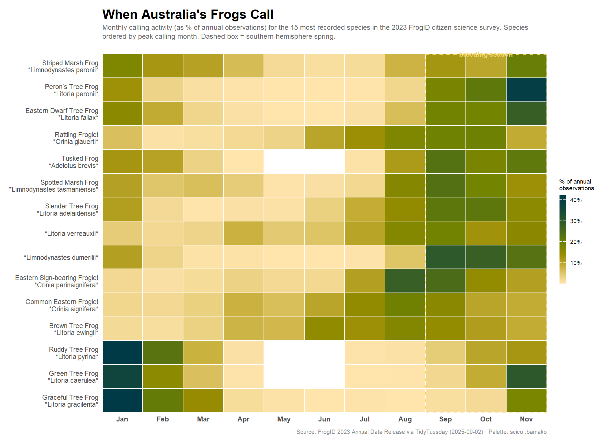
Seasonal Calling Phenology: When Do Australia’s Frogs Sing?

Frog calling is tightly coupled to breeding: males call to attract females, so call frequency spikes during the breeding season. In Australia, this creates a stark biogeographic divide:

Note

The north-south seasonal split. Tropical frogs in Queensland and the Northern Territory breed during the wet season (November–April), triggered by monsoon rains. Temperate frogs in NSW, Victoria, and South Australia breed in spring and early summer (August–November), responding to warming temperatures. The FrogID data, collected across 2023, captures both signals simultaneously.

Species richness vs. observation effort by state

state_richness <- frog_data %>%
  group_by(stateProvince) %>%
  summarise(
    n_species = n_distinct(scientificName),
    n_obs     = n(),
    .groups   = "drop"
  ) %>%
  arrange(desc(n_species))

cat("Species richness and observation effort by state:\n")
Species richness and observation effort by state:
print(state_richness)
# A tibble: 9 × 3
  stateProvince                n_species n_obs
  <chr>                            <int> <int>
1 Queensland                          96 23334
2 New South Wales                     70 58749
3 Western Australia                   52 10844
4 Northern Territory                  33  2380
5 Victoria                            28 32383
6 South Australia                     20  4158
7 Australian Capital Territory        12  2082
8 Tasmania                            11  2562
9 Other Territories                    8   129

Queensland has 96 unique species — more than triple Victoria’s 28 — yet NSW generates 2.5× more observations. This gap between where frogs are and where people are looking is the classic citizen-science sampling bias. The FrogID team explicitly accounts for this in their conservation analyses.

Constructing the seasonal calling calendar

# Filter frog_names to binomial species only to avoid genus-level many-to-many join
frog_names_sp <- frog_names %>%
  filter(str_detect(scientificName, " ")) %>%
  select(scientificName, commonName) %>%
  distinct(scientificName, .keep_all = TRUE)

# Identify top 15 species by observation count
top15_species <- frog_data %>%
  count(scientificName, sort = TRUE) %>%
  head(15) %>%
  pull(scientificName)

cat("Top 15 species selected for heatmap:\n")
Top 15 species selected for heatmap:
print(top15_species)
 [1] "Crinia signifera"           "Limnodynastes peronii"     
 [3] "Litoria fallax"             "Litoria peronii"           
 [5] "Limnodynastes tasmaniensis" "Litoria ewingii"           
 [7] "Litoria verreauxii"         "Crinia parinsignifera"     
 [9] "Limnodynastes dumerilii"    "Litoria caerulea"          
[11] "Crinia glauerti"            "Adelotus brevis"           
[13] "Litoria adelaidensis"       "Litoria gracilenta"        
[15] "Litoria pyrina"            
# Build monthly proportion matrix for top 15 species
monthly_matrix <- frog_data %>%
  filter(scientificName %in% top15_species) %>%
  mutate(month_num = month(eventDate)) %>%
  count(scientificName, month_num) %>%
  group_by(scientificName) %>%
  mutate(pct = n / sum(n)) %>%
  ungroup()

# Verify data integrity
cat(sprintf("\nmonthly_matrix: %d rows, %d cols\n", nrow(monthly_matrix), ncol(monthly_matrix)))

monthly_matrix: 159 rows, 4 cols
stopifnot("Plot data has 0 rows" = nrow(monthly_matrix) > 0)

# Quick sanity check on proportions
cat("Row sums per species (should all be ~1.0):\n")
Row sums per species (should all be ~1.0):
monthly_matrix %>%
  group_by(scientificName) %>%
  summarise(total_pct = sum(pct)) %>%
  print(n = 15)
# A tibble: 15 × 2
   scientificName             total_pct
   <chr>                          <dbl>
 1 Adelotus brevis                    1
 2 Crinia glauerti                    1
 3 Crinia parinsignifera              1
 4 Crinia signifera                   1
 5 Limnodynastes dumerilii            1
 6 Limnodynastes peronii              1
 7 Limnodynastes tasmaniensis         1
 8 Litoria adelaidensis               1
 9 Litoria caerulea                   1
10 Litoria ewingii                    1
11 Litoria fallax                     1
12 Litoria gracilenta                 1
13 Litoria peronii                    1
14 Litoria pyrina                     1
15 Litoria verreauxii                 1
# Determine peak calling month for each species (for ordering)
peak_month <- monthly_matrix %>%
  group_by(scientificName) %>%
  slice_max(pct, n = 1, with_ties = FALSE) %>%
  select(scientificName, peak_month = month_num)

# Join common names
monthly_matrix <- monthly_matrix %>%
  left_join(frog_names_sp, by = "scientificName") %>%
  left_join(peak_month, by = "scientificName") %>%
  mutate(
    # Use common name where available; fall back to italicised scientific name
    display_name = case_when(
      !is.na(commonName) & commonName != "—" ~
        paste0(commonName, "\n*", scientificName, "*"),
      TRUE ~
        paste0("*", scientificName, "*")
    ),
    # Order species by peak calling month
    display_name = fct_reorder(display_name, peak_month),
    month_abbr = factor(
      month.abb[month_num],
      levels = month.abb
    )
  )

cat("\nmonthly_matrix after join and mutate: ", nrow(monthly_matrix), "rows\n")

monthly_matrix after join and mutate:  159 rows

Visualisation: The Frog Calling Calendar

# Palette: scico::bamako (sequential, unused)
# Low = dark navy/purple (quiet month), High = warm cream/gold (peak calling)

p <- ggplot2::ggplot(
  monthly_matrix,
  ggplot2::aes(x = month_abbr, y = display_name, fill = pct)
) +
  ggplot2::geom_tile(colour = "white", linewidth = 0.4) +
  # Annotate the spring and wet-season peaks
  ggplot2::annotate(
    "rect",
    xmin = 8.5, xmax = 11.5,
    ymin = 0.5, ymax = 15.5,
    fill = NA, colour = "#F5D76E", linewidth = 0.7, linetype = "dashed",
    alpha = 0.5
  ) +
  ggplot2::annotate(
    "text",
    x = 10, y = 15.7,
    label = "Southern spring\nbreeding season",
    colour = "#F5D76E", size = 3, fontface = "bold", hjust = 0.5
  ) +
  paletteer::scale_fill_paletteer_c(
    "scico::bamako",
    direction  = -1,
    labels     = scales::label_percent(accuracy = 1),
    name       = "% of annual\nobservations",
    guide      = ggplot2::guide_colorbar(
      barwidth  = 0.6,
      barheight = 8,
      title.position = "top"
    )
  ) +
  ggplot2::scale_x_discrete(expand = ggplot2::expansion(0, 0)) +
  ggplot2::scale_y_discrete(expand = ggplot2::expansion(0, 0)) +
  ggplot2::labs(
    title    = "When Australia's Frogs Call",
    subtitle = "Monthly calling activity (as % of annual observations) for the 15 most-recorded species in the 2023 FrogID citizen-science survey.\nSpecies ordered by peak calling month. Dashed box = southern hemisphere spring.",
    x        = NULL,
    y        = NULL,
    caption  = "Source: FrogID 2023 Annual Data Release via TidyTuesday (2025-09-02) · Palette: scico::bamako"
  ) +
  ggplot2::theme_minimal(base_size = 11) +
  ggplot2::theme(
    plot.title         = ggplot2::element_text(face = "bold", size = 17, margin = ggplot2::margin(b = 4)),
    plot.subtitle      = ggtext::element_textbox_simple(
                           size = 9, colour = "grey40",
                           margin = ggplot2::margin(b = 12), lineheight = 1.3
                         ),
    plot.caption       = ggplot2::element_text(colour = "grey55", size = 7.5, margin = ggplot2::margin(t = 8)),
    axis.text.y        = ggtext::element_markdown(size = 8.5, hjust = 1),
    axis.text.x        = ggplot2::element_text(size = 9, face = "bold"),
    panel.grid         = ggplot2::element_blank(),
    legend.title       = ggplot2::element_text(size = 8),
    legend.text        = ggplot2::element_text(size = 7.5),
    plot.margin        = ggplot2::margin(12, 16, 12, 12)
  )

p

Final thoughts and takeaways

The heatmap makes a few things immediately clear:

1. Spring is frog season — for most species. The dashed box covering August–November captures the peak calling period for the majority of the top-15 species. This aligns with the southern hemisphere spring, when temperatures warm and rains arrive across eastern Australia. Crinia signifera (Common Eastern Froglet), which alone accounts for 25% of all observations, is remarkably evenly spread across the year but shows a sharp November peak.

2. The tropical outliers stand out. Uperoleia species and Queensland-heavy frogs (appearing lower in the ordered list) show relatively flat or early-year distributions, hinting at the wet-season breeding calendar of tropical Australia — though the citizen-science sampling bias toward NSW blunts this signal in the aggregate data.

3. Citizen science has a seasonality of its own. The November surge isn’t only frogs calling more — it’s also people going outside more. Disentangling phenological signal from observer effort is a persistent challenge in FrogID analyses. The research team publishes annual corrections for this bias, which is partly why FrogID requires expert acoustic verification rather than relying solely on observer labels.

4. 186 species in a single year is remarkable — and not enough. The 2023 dataset captures less than three-quarters of Australia’s 257 native frog species. Many threatened species are either in remote areas with few citizen scientists or have such small remaining populations that detection is rare. The FrogID app is actively working to close this gap, but it also underlines why the 33,000+ Crinia signifera records coexist with species recorded only once or twice in the entire dataset.

Tip

For your own exploration: The latitude and longitude fields in frogID_data are rich but deliberately coarsened (10,000m uncertainty buffers) for sensitive species. Even so, mapping species range limits — particularly the northern boundary of temperate species or the southern edge of tropical ones — against the calling calendar would be a compelling follow-up.