What does the macronutrient composition of recipes reveal about culinary traditions? Analyzing 2,200+ cuisine-tagged Allrecipes dishes to map the fat-carb-protein fingerprint of 35 global food cultures.
This week’s dataset features recipe data from Allrecipes.com, sourced through the tastyR R package. Two complementary tables are provided: all_recipes — 14,426 recipes with nutritional facts (calories, fat, carbs, protein), cooking times, ratings, and review counts — and cuisines — 2,218 recipes tagged by country or regional origin with the same nutritional and timing fields. Together they offer a rare window into how culinary traditions differ across macronutrient composition, cooking effort, and community reception.
Suggested questions from the dataset authors:
Which authors are most prolific, and do top recipe creators achieve higher ratings?
Is there a correlation between preparation time and average rating?
Which cuisines receive the highest average ratings and review engagement?
Which recipes are most “actionable” — high ratings with minimal total prep and cook time?
Loading necessary packages
My handy booster pack that allows me to install (if needed) and load my usual and favorite packages, as well as some helpful functions.
A few things stand out immediately. Ratings cluster high — the median avg_rating is 4.6 out of 5.0, with the 25th percentile already at 4.4. This is typical of self-selected recipe sites: unpopular recipes disappear, survivors skew positive. Review counts are highly right-skewed: the median recipe has just 26 ratings but the mean is 103, pulled up by a long tail of viral hits. Cooking times show enormous spread — median total time is 55 minutes, but the 90th percentile is 4+ hours, with slow-cooker braises and overnight doughs pulling the tail out.
The cuisines table mirrors the all_recipes structure but adds the country column. It spans 49 distinct cuisine labels with roughly 25–67 recipes each. Nutritional distributions look similar to the main table — median calories around 300, fat heavy relative to protein. The avg_rating distribution here is slightly higher (median 4.6, mean closer to 4.5 after accounting for NA), consistent with the general recipes dataset.
# A tibble: 49 × 2
   country                          n
   <chr>                        <int>
 1 Brazilian                       67
 2 Canadian                        67
 3 Filipino                        66
 4 Australian and New Zealander    65
 5 Chinese                         65
 6 Cuban                           65
 7 French                          65
 8 Indian                          65
 9 Russian                         65
10 Italian                         64
11 Cajun and Creole                63
12 Japanese                        63
13 Soul Food                       63
14 German                          62
15 Greek                           62
16 Thai                            62
17 Vietnamese                      62
18 Amish and Mennonite             61
19 Jewish                          61
20 Polish                          61
21 Spanish                         61
22 Puerto Rican                    60
23 Korean                          56
24 Tex-Mex                         55
25 Portuguese                      53
26 Lebanese                        51
27 Southern Recipes                50
28 Persian                         45
29 Jamaican                        43
30 Peruvian                        38
31 Scandinavian                    38
32 Turkish                         36
33 Danish                          33
34 Swedish                         31
35 Argentinian                     30
36 Norwegian                       26
37 Pakistani                       25
38 Indonesian                      24
39 Malaysian                       24
40 Israeli                         23
41 Austrian                        22
42 Chilean                         22
43 Dutch                           22
44 South African                   19
45 Finnish                         18
46 Bangladeshi                     12
47 Colombian                       11
48 Swiss                           10
49 Belgian                          6
The 49 cuisines are roughly balanced, most with 50–67 recipes. Smaller samples appear toward the bottom (Israeli: 23, Nigerian: 14). For the main analysis I’ll restrict to cuisines with at least 30 recipes to ensure stable medians.
Macronutrient Fingerprints of Global Cuisines
The central question: does cuisine identity translate into nutritionally distinct recipes? Each culinary tradition carries embedded constraints — available ingredients, historical influences, climate, and cultural preferences around protein sources, starchy staples, and cooking fats. If those patterns are real, they should appear in the macronutrient composition of typical dishes.
To test this, I convert raw grams of fat, carbohydrates, and protein into caloric contributions using standard Atwater factors (fat: 9 kcal/g; carbohydrate and protein: 4 kcal/g each), then express each macro as a share of total macro-derived calories per recipe. Taking the median within each cuisine gives a stable central tendency that resists individual outliers (e.g., one unusually rich French pastry won’t define French cuisine).
# Global medians across all qualifying recipesglobal_fat <-median(macro_by_recipe$pct_fat)global_carb <-median(macro_by_recipe$pct_carb)global_prot <-median(macro_by_recipe$pct_protein)cat(sprintf("Global macro medians:\n Fat: %.1f%%\n Carbohydrate: %.1f%%\n Protein: %.1f%%\n", global_fat, global_carb, global_prot))
Global macro medians:
  Fat: 43.9%
  Carbohydrate: 37.9%
  Protein: 14.9%
# Top and bottom by proteincuisine_macros %>% dplyr::select(country, n, med_pct_fat, med_pct_carb, med_pct_protein, med_calories) %>% dplyr::mutate(dplyr::across(dplyr::starts_with("med_pct"), ~round(.x, 1))) %>%print(n =35)
A note on methodology. These figures represent the median recipe in each cuisine category, not the average diet of people in those countries. Allrecipes skews toward home cooking, special occasion dishes, and recipes submitted by users in English-speaking markets. The data reflects what Allrecipes users associate with each culinary label — a useful proxy, but not a direct measure of traditional foodways.
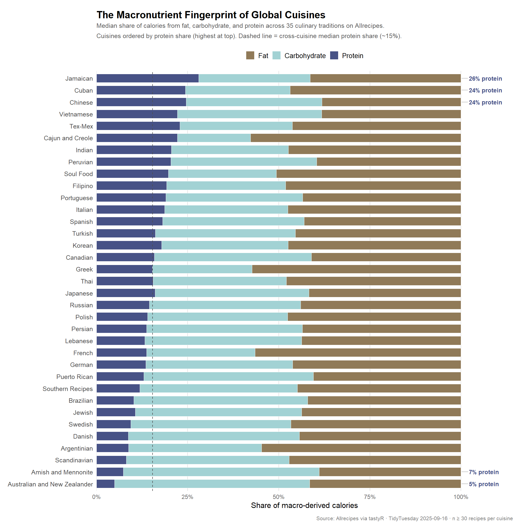
The spread is striking. Jamaican, Cuban, and Chinese recipes sit at the top for protein share (26%, 24%, and 24% respectively), driven by meat-forward dishes like jerk chicken, ropa vieja, and stir-fries. At the other extreme, Australian/New Zealand and Amish/Mennonite cuisines are the most carbohydrate-dominant (53% of calories from carbs), reflecting traditions rich in baked goods, pies, and grain-based staples. Cajun/Creole and Greek recipes stand out as the most fat-heavy, consistent with generous use of butter, cream, olive oil, and rich cuts of meat.
Hero Visualization
# Build factor order: cuisines sorted by protein % (ascending so top protein = top of chart)protein_order <- cuisine_macros %>% dplyr::arrange(med_pct_protein) %>% dplyr::pull(country)# Pivot to long format for stacked barmacro_long <- cuisine_macros %>% dplyr::select(country, med_pct_fat, med_pct_carb, med_pct_protein) %>% tidyr::pivot_longer(cols = dplyr::starts_with("med_pct"),names_to ="macro",values_to ="pct" ) %>% dplyr::mutate(macro = dplyr::case_when( macro =="med_pct_fat"~"Fat", macro =="med_pct_carb"~"Carbohydrate", macro =="med_pct_protein"~"Protein" ),macro =factor(macro, levels =c("Fat", "Carbohydrate", "Protein")),country =factor(country, levels = protein_order) )cat(sprintf("macro_long: %d rows, %d cols\n", nrow(macro_long), ncol(macro_long)))
macro_long: 105 rows, 3 cols
stopifnot("Plot data is empty"=nrow(macro_long) >0)# Palette: IslamicArt::samarqand — earthy brown (fat), soft aqua (carbs), deep indigo (protein)samarqand_pal <- paletteer::paletteer_d("IslamicArt::samarqand")macro_colors <-c("Fat"=as.character(samarqand_pal[2]), # #907A58 warm earth"Carbohydrate"=as.character(samarqand_pal[5]), # #A2D2D4 soft aqua"Protein"=as.character(samarqand_pal[6]) # #475286 deep indigo)# Annotation data: label highest- and lowest-protein cuisineslabel_cuisines <-c("Jamaican", "Cuban", "Chinese","Amish and Mennonite", "Australian and New Zealander")annotation_df <- cuisine_macros %>% dplyr::filter(country %in% label_cuisines) %>% dplyr::mutate(country =factor(country, levels = protein_order),label =sprintf("%.0f%% protein", round(med_pct_protein, 0)) )p <- macro_long %>% ggplot2::ggplot(ggplot2::aes(x = pct, y = country, fill = macro)) + ggplot2::geom_col(position ="fill", width =0.72, colour ="white", linewidth =0.2) +# Reference line: global median protein share ggplot2::geom_vline(xintercept =1- (global_fat + global_carb) / (global_fat + global_carb + global_prot),colour ="grey30", linetype ="dashed", linewidth =0.5 ) +# Protein % labels on highlighted cuisines ggrepel::geom_text_repel(data = annotation_df, ggplot2::aes(x =1, y = country, label = label),inherit.aes =FALSE,hjust =0,nudge_x =0.02,size =3.2,colour ="#475286",fontface ="bold",direction ="y",segment.size =0.3,segment.colour ="grey50" ) + ggplot2::scale_x_continuous(labels = scales::percent_format(accuracy =1),expand = ggplot2::expansion(mult =c(0, 0.12)),breaks =seq(0, 1, 0.25) ) + ggplot2::scale_fill_manual(values = macro_colors) + ggplot2::labs(title ="The Macronutrient Fingerprint of Global Cuisines",subtitle =paste0("Median share of calories from fat, carbohydrate, and protein across 35 culinary traditions on Allrecipes.\n","Cuisines ordered by protein share (highest at top). Dashed line = cross-cuisine median protein share (~15%)." ),x ="Share of macro-derived calories",y =NULL,fill =NULL,caption ="Source: Allrecipes via tastyR · TidyTuesday 2025-09-16 · n ≥ 30 recipes per cuisine" ) + ggplot2::theme_minimal(base_size =11.5) + ggplot2::theme(plot.title = ggtext::element_markdown(face ="bold", size =15, margin = ggplot2::margin(b =4)),plot.subtitle = ggplot2::element_text(size =9.5, colour ="grey35", lineheight =1.35,margin = ggplot2::margin(b =12)),plot.caption = ggplot2::element_text(size =8, colour ="grey50",margin = ggplot2::margin(t =10)),legend.position ="top",legend.key.size = ggplot2::unit(0.9, "lines"),legend.text = ggplot2::element_text(size =10),axis.text.y = ggplot2::element_text(size =9.5),axis.text.x = ggplot2::element_text(size =9, colour ="grey40"),panel.grid.minor = ggplot2::element_blank(),panel.grid.major.y = ggplot2::element_blank(),panel.grid.major.x = ggplot2::element_line(colour ="grey88"),plot.margin = ggplot2::margin(16, 24, 12, 12) )p
Final thoughts and takeaways
The macronutrient fingerprint of a cuisine is not random noise — it reflects real structural differences in culinary logic. The high-protein cluster at the top (Jamaican, Cuban, Chinese, Vietnamese) skews heavily toward meat-centric main courses: jerk preparations, braised pork, stir-fried proteins, and pho. These traditions put the protein source at the center of the plate and build everything else around it.
The carbohydrate-dominant end of the spectrum tells a different story. Australian and New Zealand recipes on Allrecipes lean disproportionately toward baked goods — pavlova, lamingtons, Anzac biscuits — categories where flour, sugar, and oats dominate. Amish and Mennonite cooking reflects a tradition grounded in stretching protein-scarce ingredients with starches: potato dishes, noodle casseroles, and pies. Neither cuisine is “less healthy” in some absolute sense, but the carb emphasis is a real feature of what gets submitted and rated in those categories.
Cajun/Creole and Greek stand out as the most fat-heavy cuisines, both exceeding 55% of calories from fat. For Cajun cooking this tracks with the heavy use of butter and roux in étouffée, gumbo, and jambalaya. For Greek cuisine it reflects olive oil used generously in everything from phyllo pastry to moussaka.
A few caveats worth noting:
Allrecipes users tend to submit and rate celebratory or indulgent dishes more than everyday meals, which likely inflates calorie counts and fat percentages across the board.
Cuisine tags are assigned by Allrecipes editors, not by cultural experts — the “Australian and New Zealand” category almost certainly oversamples European-descended baking traditions relative to Indigenous or Pacific Island foodways.
The dataset captures a snapshot of user-submitted content through mid-2025; trending dietary styles (keto, plant-based) may skew toward recent submission dates.
Despite these limitations, the broad patterns are robust: culinary tradition does leave a legible macronutrient signature, and that signature is meaningful enough to distinguish 35 cuisines in a way that largely matches intuition about each food culture’s defining characteristics.
Render note: Render locally once with quarto render before committing — the _freeze/ directory captures executed output and CI will not re-execute.