The dataset comes from the Fédération Internationale des Échecs (FIDE), the international governing body of chess. It includes the FIDE ratings list for August and September 2025, with information on over 200,000 rated players worldwide. Each record includes the player’s rating, federation (country), sex, official titles (if any), K-factor, and birth year. FIDE ratings use the Elo system, where a player’s number represents their expected performance relative to peers — higher is better.
This data covers the full breadth of the rated chess world, from club beginners to Magnus Carlsen at the summit.
Loading necessary packages
My handy booster pack that allows me to install (if needed) and load my usual and favorite packages, as well as some helpful functions.
raw <- tidytuesdayR::tt_load("2025-09-23")aug <- raw$fide_ratings_augustsep <- raw$fide_ratings_september
Exploratory Data Analysis
The my_skim() function is a modified version of the skimr::skim() function that returns the number of missing data points (cells as NA) as well as the inverse (e.g.: number of rows that are notNA), the count, minimum, 25%, median, 75%, max, mean, geometric mean, and standard deviation. It also generates a little ASCII histogram. Neat!
We drop the id (an internal FIDE identifier) and free-text name column before skimming, since they carry no distributional signal. The otitle and foa columns are heavily sparse in this snapshot and also excluded from the EDA profile.
August 2025 Ratings
aug %>%select(-id, -name, -otitle, -foa) %>%my_skim()
# Sex distributioncat("=== Sex distribution (August) ===\n")
=== Sex distribution (August) ===
aug %>%count(sex, sort =TRUE) %>%print()
# A tibble: 2 × 2
  sex        n
  <chr>  <int>
1 M     180258
2 F      20757
# Title distributioncat("\n=== Title distribution (August) ===\n")
=== Title distribution (August) ===
aug %>%count(title, sort =TRUE) %>%print()
# A tibble: 9 × 2
  title      n
  <chr>  <int>
1 <NA>  188366
2 FM      4762
3 IM      2433
4 CM      2073
5 GM      1306
6 WFM      825
7 WCM      652
8 WIM      413
9 WGM      185
# Top 10 federationscat("\n=== Top 10 federations by player count ===\n")
=== Top 10 federations by player count ===
aug %>%count(fed, sort =TRUE) %>%head(10) %>%print()
# A tibble: 10 × 2
   fed       n
   <chr> <int>
 1 ESP   17858
 2 IND   16445
 3 FRA   15958
 4 GER   13310
 5 RUS    7228
 6 ITA    6702
 7 POL    5946
 8 CZE    5557
 9 USA    4495
10 NED    4227
# Rating rangecat("\n=== Rating range ===\n")
=== Rating range ===
summary(aug$rating)
   Min. 1st Qu.  Median    Mean 3rd Qu.    Max.
   1400    1564    1715    1745    1886    2839
The August 2025 list contains 201,015 rated players from 167 federations. The vast majority — 188,366 (94%) — are untitled club players, forming the broad base beneath a narrow pyramid of titled masters. Males outnumber females roughly 8.7 to 1, though both sexes span the full rating range. Spain, India, and France lead in raw player count, but as we’ll see, player count alone tells a very different story from elite strength.
The Chess Title Hierarchy
FIDE’s title system is one of the clearest examples of credentialing in competitive sport. Titles are earned through a combination of rating thresholds and performance norms in qualifying tournaments:
NoteTitle thresholds (simplified)
Title
Meaning
Approx. rating threshold
GM
Grandmaster
2500+ (plus 3 GM norms)
IM
International Master
2400+ (plus 3 IM norms)
FM
FIDE Master
2300+
CM
Candidate Master
2200+
WGM
Woman Grandmaster
2300+ (women’s norm circuit)
WIM
Woman International Master
2200+
WFM
Woman FIDE Master
2100+
WCM
Woman Candidate Master
2000+
Once earned, titles are permanent — which is why some players’ current ratings sit below the threshold they originally crossed.
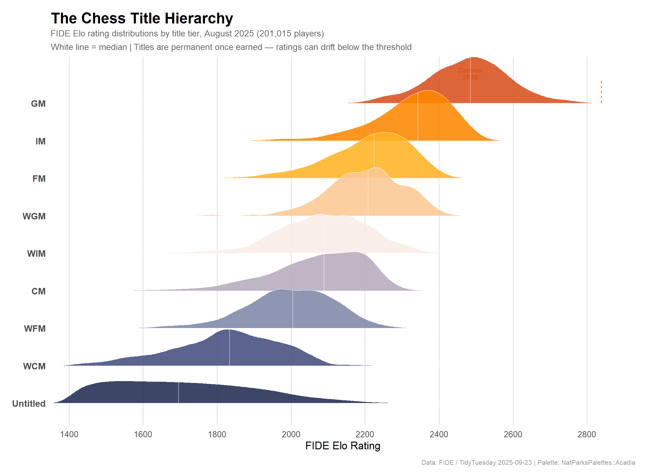
Rating distributions by title tier
# Define the canonical ordering by descending median ratingtitle_order <-c("GM", "IM", "FM", "WGM", "WIM", "CM", "WFM", "WCM", "Untitled")plot_data_tiers <- aug %>%mutate(title_clean =ifelse(is.na(title), "Untitled", title)) %>%filter(title_clean %in% title_order) %>%mutate(title_factor =factor(title_clean, levels =rev(title_order)))cat(sprintf("plot_data_tiers: %d rows, %d cols\n", nrow(plot_data_tiers), ncol(plot_data_tiers)))
plot_data_tiers: 201015 rows, 14 cols
stopifnot("Plot data has 0 rows — check filter values"=nrow(plot_data_tiers) >0)# Sanity check: medians per tiertier_medians <- plot_data_tiers %>%group_by(title_clean) %>%summarise(n =n(), median_rating =median(rating), .groups ="drop") %>%arrange(desc(median_rating))print(tier_medians)
# A tibble: 9 × 3
  title_clean      n median_rating
  <chr>        <int>         <dbl>
1 GM            1306          2484
2 IM            2433          2342
3 FM            4762          2224
4 WGM            185          2208
5 WIM            413          2090
6 CM            2073          2089
7 WFM            825          2004
8 WCM            652          1833
9 Untitled    188366          1696
# Check for all-identical medians (would indicate bad grouping)if (length(unique(tier_medians$median_rating)) ==1) {warning("All tier medians identical — check grouping logic")}
# NatParksPalettes::Acadia — 9 colors, navy-to-orange gradient# Mapping: Untitled (cool navy) → GM (warm orange-red)acadia_pal <- paletteer::paletteer_d("NatParksPalettes::Acadia")# Map palette in ascending order of title prestige# title_order = c("GM", "IM", ..., "Untitled") = high to low# rev(title_order) = c("Untitled", ..., "GM") = factor levels (bottom to top of ridge)# acadia_pal[1] = navy → "Untitled", acadia_pal[9] = orange-red → "GM"tier_colors <-setNames(as.character(acadia_pal), rev(title_order))p_ridges <- ggplot2::ggplot( plot_data_tiers, ggplot2::aes(x = rating, y = title_factor, fill = title_factor)) + ggridges::geom_density_ridges(alpha =0.88,scale =1.35,color ="white",linewidth =0.35,quantile_lines =TRUE,quantiles =2,quantile_fun = median ) + ggplot2::scale_fill_manual(values = tier_colors) + ggplot2::scale_x_continuous(limits =c(1350, 2900),breaks =seq(1400, 2800, 200),expand = ggplot2::expansion(mult =c(0, 0.02)) ) + ggplot2::annotate("text", x =2484, y =9.8,label ="Carlsen\n2839", size =2.8, color ="#D8511D",fontface ="bold", hjust =0.5, lineheight =0.9 ) + ggplot2::annotate("segment", x =2839, xend =2839, y =9, yend =9.6,color ="#D8511D", linewidth =0.5, linetype ="dashed" ) + ggplot2::labs(title ="The Chess Title Hierarchy",subtitle ="FIDE Elo rating distributions by title tier, August 2025 (201,015 players)\nWhite line = median | Titles are permanent once earned — ratings can drift below the threshold",x ="FIDE Elo Rating",y =NULL,caption ="Data: FIDE / TidyTuesday 2025-09-23 | Palette: NatParksPalettes::Acadia" ) + ggplot2::theme_minimal(base_size =13) + ggplot2::theme(legend.position ="none",plot.title = ggplot2::element_text(face ="bold", size =18, margin = ggplot2::margin(b =4)),plot.subtitle = ggplot2::element_text(color ="grey40", size =10.5, lineheight =1.3),plot.caption = ggplot2::element_text(color ="grey60", size =8, margin = ggplot2::margin(t =10)),axis.text.y = ggplot2::element_text(face ="bold", size =11),axis.text.x = ggplot2::element_text(size =10),panel.grid.minor = ggplot2::element_blank(),panel.grid.major.y = ggplot2::element_blank(),panel.grid.major.x = ggplot2::element_line(color ="grey90"),plot.margin = ggplot2::margin(15, 20, 10, 15) )p_ridges
A few things jump out immediately:
The GM distribution is remarkably tight — the interquartile range runs from roughly 2409 to 2550, a span of only 141 points. Grandmasters are densely clustered near the top of the rating scale.
Untitled players have the widest spread by far. This tier encompasses every club player from absolute beginner (1400, the FIDE floor) to talented unregistered-norm players near 2480. The long right tail reveals many strong players who simply never pursued formal title norms.
Women’s titles interleave with open titles. The WGM median (2208) sits between FM (2224) and WIM (2090), while WIM overlaps almost exactly with CM. This reflects FIDE’s design — women’s titles carry lower rating requirements, allowing the system to recognize female achievement at equivalent competitive standards within women’s events.
The gap between IM and GM is the largest between adjacent tiers — roughly 140 Elo points separating medians, compared to ~120 between FM and IM. Earning the final GM title is, by reputation, the hardest step in chess.
TipWhat’s the K-factor?
The k column (values: 10, 20, 40) is FIDE’s sensitivity dial for rating changes. Players with K=40 are new to the rating list or under 18, and their ratings adjust quickly after each game. K=20 is the standard for established players. K=10 applies to elite players rated 2400+ who have played 30+ rated games — their ratings change very slowly, as they’ve “earned” stability.
India’s Chess Revolution
The title hierarchy tells us what the system looks like globally. But hidden within the federation data is one of the most remarkable stories in modern chess: India’s ascent to the pinnacle of the game.
# Federation GM analysis — top federations by GM countfed_gm_stats <- aug %>%filter(title =="GM") %>%group_by(fed) %>%summarise(n_gm =n(),avg_gm_rating =mean(rating, na.rm =TRUE),avg_gm_bday =mean(bday, na.rm =TRUE), # proxy for GM corps age.groups ="drop" ) %>%filter(n_gm >=10) %>%arrange(desc(n_gm))cat(sprintf("fed_gm_stats: %d rows, %d cols\n", nrow(fed_gm_stats), ncol(fed_gm_stats)))
fed_gm_stats: 42 rows, 4 cols
stopifnot("Federation GM data has 0 rows"=nrow(fed_gm_stats) >0)# Sanity check: ratings should vary by federationif (length(unique(round(fed_gm_stats$avg_gm_rating))) ==1) {warning("All avg GM ratings identical — check grouping logic")}# Exclude FID (FIDE stateless players — international citizens w/o federation)fed_gm_stats <- fed_gm_stats %>%filter(fed !="FID")# Add India flag for highlightingfed_gm_stats <- fed_gm_stats %>%mutate(is_india = fed =="IND")print(fed_gm_stats %>%arrange(desc(n_gm)) %>%head(15))
# Top 20 federations by GM countplot_data_feds <- fed_gm_stats %>%arrange(desc(n_gm)) %>%head(20)cat(sprintf("plot_data_feds: %d rows\n", nrow(plot_data_feds)))
plot_data_feds: 20 rows
stopifnot("Federation scatter data has 0 rows"=nrow(plot_data_feds) >0)p_feds <- ggplot2::ggplot( plot_data_feds, ggplot2::aes(x = avg_gm_bday,y = avg_gm_rating,size = n_gm,color = is_india )) + ggplot2::geom_point(alpha =0.82) + ggrepel::geom_text_repel( ggplot2::aes(label = fed),size =3.2,fontface ="bold",min.segment.length =0.2,box.padding =0.5,color ="grey20",show.legend =FALSE ) + ggplot2::scale_color_manual(values =c("TRUE"="#D8511D", "FALSE"="#8087AA"),guide ="none" ) + ggplot2::scale_size_continuous(name ="Number of GMs",range =c(3, 14),breaks =c(10, 25, 50, 75) ) + ggplot2::scale_x_continuous(name ="Average GM birth year",breaks =seq(1975, 2000, 5),labels =function(x) paste0(x) ) + ggplot2::scale_y_continuous(name ="Average GM Elo rating",breaks =seq(2420, 2560, 20) ) + ggplot2::annotate("text",x =1995.8, y =2530,label ="India: youngest & strongest\nGM corps among major nations",color ="#D8511D", size =3.3, fontface ="bold",hjust =0, lineheight =1.1 ) + ggplot2::labs(title ="India's GMs are younger — and stronger",subtitle ="Average Elo rating vs. average birth year of Grandmasters, by federation (top 20 by GM count)\nBubble size = number of GMs | India highlighted in orange",caption ="Data: FIDE / TidyTuesday 2025-09-23 | Palette: NatParksPalettes::Acadia (accent colors)" ) + ggplot2::theme_minimal(base_size =13) + ggplot2::theme(plot.title = ggplot2::element_text(face ="bold", size =16, margin = ggplot2::margin(b =4)),plot.subtitle = ggplot2::element_text(color ="grey40", size =10, lineheight =1.3),plot.caption = ggplot2::element_text(color ="grey60", size =8, margin = ggplot2::margin(t =10)),panel.grid.minor = ggplot2::element_blank(),legend.position ="bottom",plot.margin = ggplot2::margin(15, 20, 10, 15) )p_feds
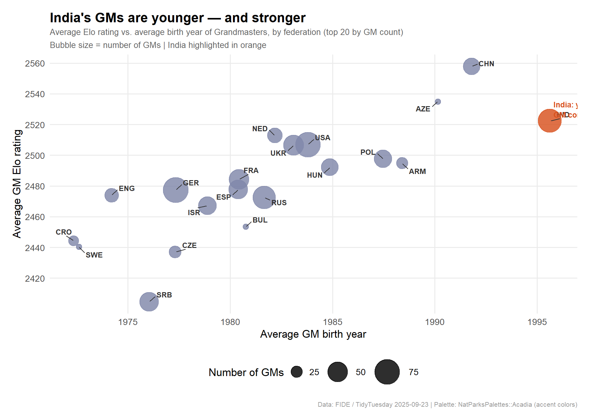
The scatter tells a clear story. India sits in the upper-right quadrant — its GMs average a birth year around 1996 (the youngest cohort among any major chess nation) while also carrying the highest average rating among the top-ten GM-producing countries. Germany and the USA have more GMs, but their cohorts are older (averaging birth years of 1977 and 1984 respectively). England’s GMs, for context, average a birth year of 1974.
ImportantThe Indian Chess Boom in context
In 2024, D. Gukesh (born 2006) became the youngest World Chess Champion in history, defeating Ding Liren in Singapore. At the time of this dataset, Praggnanandhaa R (born 2005) and Erigaisi Arjun (born 2003) ranked 4th and 5th in the world respectively — alongside Gukesh at 6th. Three of the world’s top six players are Indian teenagers or early-twenty-somethings.
India’s current GM corps (avg. birth year 1996) is strikingly young because the pipeline is recent: FIDE-rated chess only reached mass participation in India in the 2000s, catalyzed by Viswanathan Anand’s world title and government investment in chess coaching infrastructure. The country is now producing grandmasters faster than any other nation.
# Verify: top 10 players in September ratingscat("=== Top 10 players, September 2025 ===\n")
# A tibble: 10 × 5
   name              fed   title rating games
   <chr>             <chr> <chr>  <dbl> <dbl>
 1 Carlsen, Magnus   NOR   GM      2839     0
 2 Nakamura, Hikaru  USA   GM      2807     0
 3 Caruana, Fabiano  USA   GM      2789     9
 4 Praggnanandhaa R  IND   GM      2785     9
 5 Erigaisi Arjun    IND   GM      2771     9
 6 Gukesh D          IND   GM      2767     9
 7 So, Wesley        USA   GM      2756     9
 8 Firouzja, Alireza FRA   GM      2754     9
 9 Wei, Yi           CHN   GM      2753     0
10 Keymer, Vincent   GER   GM      2751     9
# India's share of top 100india_top100 <- sep %>%arrange(desc(rating)) %>%mutate(rank =row_number()) %>%filter(rank <=100) %>%count(fed, name ="n_top100") %>%arrange(desc(n_top100)) %>%head(10)cat("\n=== Federations represented in top 100 (September) ===\n")
=== Federations represented in top 100 (September) ===
print(india_top100)
# A tibble: 10 × 2
   fed   n_top100
   <chr>    <int>
 1 USA         12
 2 IND         11
 3 CHN          6
 4 RUS          6
 5 UZB          5
 6 AZE          4
 7 ENG          4
 8 FID          4
 9 GER          4
10 ESP          3
Palette log update
Final thoughts and takeaways
The FIDE rating database, at first glance, is just a giant spreadsheet of numbers. But structurally it’s a map of a global competitive meritocracy — one of the few human domains where rank is both objectively computed and universally legible.
A few takeaways from this analysis:
The title system is a clear hierarchy. The ridge plot shows that FIDE titles genuinely carve the player population into meaningful skill tiers, not arbitrary labels. The gaps between adjacent title medians are real and significant — crossing each threshold represents a qualitatively different level of play. The GM boundary, in particular, sits at a rating level that fewer than 1-in-150 rated players ever reach.
India is the dominant story in elite chess right now. The combination of the youngest and highest-rated GM corps among major nations is not a coincidence. It reflects a pipeline effect: when Anand’s world titles inspired a generation in the late 1990s and 2000s, coaching infrastructure followed. That cohort is now in its prime — and the next wave is already here.
Most of the chess world is untitled — and that’s fine. The 188,000+ untitled players in this dataset aren’t failures of the system. They represent the actual community that makes competitive chess viable: people who play in local clubs, online arenas, and weekend tournaments for the love of the game. Their spread across the 1400–2400 range shows that recreational chess and elite chess coexist on the same rating axis, connected by a shared numeric language.
One caveat: this dataset only covers the FIDE-registered universe. An enormous number of casual chess.com and Lichess players never enter the FIDE system at all — the 1400 floor here is not the true floor of global chess participation.