Tidy Tuesday: Crane Observations at Lake Hornborgasjön, Sweden (1994–2024)

Thirty years of Eurasian crane migration counts at Sweden’s most celebrated staging lake reveal a remarkable fivefold population recovery — and a 2023 fall season that rewrote the record books.

Preface

From TidyTuesday repository.

This dataset documents crane counts at Lake Hornborgasjön in Sweden spanning 1994–2024. The field station has tracked migrations for over 30 years, counting birds during spring and fall passages. Dataset curated by Carl Borstell from the Hornborgasjön field station’s official statistics.

Suggested questions from the repository:

1. How have crane counts changed across the 30-year period (1994–2024)?
2. When during the year are the largest crane congregations observed?
3. Can weather patterns predict or correlate with crane arrivals?

Loading necessary packages

My handy booster pack that allows me to install (if needed) and load my usual and favorite packages, as well as some helpful functions.

# Packages ----------------------------------------------------------------

{
  # Install pak if it's not already installed
  if (!requireNamespace("pak", quietly = TRUE)) {
    install.packages(
      "pak",
      repos = sprintf(
        "https://r-lib.github.io/p/pak/stable/%s/%s/%s",
        .Platform$pkgType,
        R.Version()$os,
        R.Version()$arch
      )
    )
  }

  # CRAN Packages ----
  install_booster_pack <- function(package, load = TRUE) {
    for (pkg in package) {
      if (!requireNamespace(pkg, quietly = TRUE)) {
        pak::pkg_install(pkg)
      }
      if (load) {
        library(pkg, character.only = TRUE)
      }
    }
  }

  booster_pack <- c(
    ### IO ----
    'fs',
    'here',
    'janitor',
    'rio',
    'tidyverse',

    ### EDA ----
    'skimr',

    ### Plot ----
    'paletteer',           # Color palette collection
    'ggridges',            # Ridgeline / joy plots
    'ggrepel',             # Non-overlapping labels
    'patchwork',           # Multi-panel layouts

    ### Misc ----
    'tidytuesdayR'
  )

  install_booster_pack(package = booster_pack, load = TRUE)
  rm(install_booster_pack, booster_pack)

  # Custom Functions ----

  `%ni%` <- Negate(`%in%`)

  geometric_mean <- function(x) {
    exp(mean(log(x[x > 0]), na.rm = TRUE))
  }

  my_skim <- skim_with(
    numeric = sfl(
      n = length,
      min = ~ min(.x, na.rm = T),
      p25 = ~ stats::quantile(., probs = .25, na.rm = TRUE, names = FALSE),
      med = ~ median(.x, na.rm = T),
      p75 = ~ stats::quantile(., probs = .75, na.rm = TRUE, names = FALSE),
      max = ~ max(.x, na.rm = T),
      mean = ~ mean(.x, na.rm = T),
      geo_mean = ~ geometric_mean(.x),
      sd = ~ stats::sd(., na.rm = TRUE),
      hist = ~ inline_hist(., 5)
    ),
    append = FALSE
  )
}

Load raw data from package

raw <- tidytuesdayR::tt_load('2025-09-30')

cranes <- raw$cranes

Exploratory Data Analysis

The my_skim() function is a modified version of the skimr::skim() function that returns the number of missing data points (cells as NA) as well as the inverse (e.g.: number of rows that are not NA), the count, minimum, 25%, median, 75%, max, mean, geometric mean, and standard deviation. It also generates a little ASCII histogram. Neat!

cranes

cranes %>%
  select(date, observations) %>%
  my_skim()

Data summary

Name	Piped data
Number of rows	1548
Number of columns	2
_______________________
Column type frequency:
Date	1
numeric	1
________________________
Group variables	None

Variable type: Date

skim_variable	n_missing	complete_rate	min	max	median	n_unique
date	0	1	1994-03-24	2024-10-03	2011-03-21	1546

Variable type: numeric

skim_variable	n_missing	complete_rate	n	min	p25	med	p75	max	mean	geo_mean	sd	hist
observations	161	0.9	1548	0	1645	4500	8935	27300	6063.49	3028.25	5537	▇▃▂▁▁

# Inspect the categorical fields
cranes %>% count(comment, sort = TRUE)

# A tibble: 8 × 2
  comment                   n
  <chr>                 <int>
1 <NA>                   1358
2 Canceled/No count       146
3 Uncertain count          22
4 Severe interference       7
5 Last count of season      6
6 Bad weather               4
7 Record observation        3
8 First count of season     2

cranes %>% count(weather_disruption)

# A tibble: 2 × 2
  weather_disruption     n
  <lgl>              <int>
1 FALSE               1507
2 TRUE                  41

The dataset contains 1,548 observation records spanning March 1994 through October 2024 — 31 spring and fall migration seasons at Lake Hornborgasjön. A few structural features stand out immediately:

• 161 missing observation counts (10.4% of rows): nearly all correspond to canceled counts due to bad weather, severe interference, or no-shows. These are data-absent days, not zero-crane days, and should be excluded from analysis.
• Crane counts span 0 to 27,300 with a median of 4,500 and a mean of 6,063 — the right-skewed distribution is typical of wildlife staging sites where peak days pull the mean well above the typical day.
• Only 41 weather disruptions flagged across three decades, suggesting the field station operated reliably through most conditions.
• Three “Record observation” comments all date to September 2023 — a remarkable cluster that flags an unusual fall season we’ll examine closely.

# Add time components used throughout the analysis
cranes <- cranes %>%
  mutate(
    year        = lubridate::year(date),
    month       = lubridate::month(date),
    month_name  = lubridate::month(date, label = TRUE, abbr = TRUE),
    day_of_year = lubridate::yday(date),
    season      = case_when(
      month %in% 3:5  ~ "Spring",
      month %in% 9:11 ~ "Fall",
      TRUE            ~ "Summer"
    )
  )

# Season-level summary
cranes %>%
  filter(!is.na(observations)) %>%
  group_by(season) %>%
  dplyr::summarise(
    n_counts      = dplyr::n(),
    median_obs    = median(observations),
    max_obs       = max(observations),
    mean_obs      = round(mean(observations))
  )

# A tibble: 3 × 5
  season n_counts median_obs max_obs mean_obs
  <chr>     <int>      <dbl>   <dbl>    <dbl>
1 Fall        264       5570   24300     6691
2 Spring     1050       4600   27300     6190
3 Summer       73       1780    5710     1978

Spring dominates: 1,050 of the 1,387 valid observation days fall in March–May, with a median of 4,600 cranes. Fall provides 264 valid counts (median: 5,570), while the small number of August “summer” counts (n=73) mostly capture early arriving birds before the main fall passage.

Domain Analysis: Three Decades of Recovery

Note

Lake Hornborgasjön and the Crane’s Return

Lake Hornborgasjön in Västergötland, Sweden, was once one of the country’s most biodiverse wetlands. A century of drainage attempts to convert it to farmland collapsed its ecology. In the late 1980s, a major restoration project raised the water level by 1.5 meters, recovering shallow reed beds and open water habitat. The Eurasian crane (Grus grus) responded almost immediately — counts began in 1994 as the habitat re-established itself.

Today Hornborgasjön hosts one of Europe’s largest crane congregations during spring migration, often attracting more than 20,000 birds at peak. The Swedish “cranewatch” webcam draws hundreds of thousands of online viewers every spring.

Annual peak counts: a population story

annual_peaks <- cranes %>%
  filter(!is.na(observations)) %>%
  dplyr::group_by(year) %>%
  dplyr::summarise(
    n_days     = dplyr::n(),
    peak_count = max(observations),
    median_obs = median(observations),
    peak_date  = date[which.max(observations)],
    peak_doy   = lubridate::yday(peak_date),
    peak_month = lubridate::month(peak_date, label = TRUE)
  ) %>%
  dplyr::ungroup()

cat(sprintf("annual_peaks: %d rows, %d cols\n", nrow(annual_peaks), ncol(annual_peaks)))

annual_peaks: 31 rows, 7 cols

stopifnot("annual_peaks has 0 rows" = nrow(annual_peaks) > 0)

print(annual_peaks, n = 31)

# A tibble: 31 × 7
    year n_days peak_count median_obs peak_date  peak_doy peak_month
   <dbl>  <int>      <dbl>      <dbl> <date>        <dbl> <ord>     
 1  1994     28       4992      3100  1994-04-08       98 Apr       
 2  1995     37       5280      1907  1995-04-17      107 Apr       
 3  1996     27       5880      2150  1996-04-18      109 Apr       
 4  1997     34       6860      3050  1997-04-09       99 Apr       
 5  1998     36       8625      4932. 1998-04-15      105 Apr       
 6  1999     31       7800      3775  1999-04-07       97 Apr       
 7  2000     33       8920      6850  2000-04-09      100 Apr       
 8  2001     35       6750      2675  2001-04-19      109 Apr       
 9  2002     53       8760      3800  2002-04-04       94 Apr       
10  2003     43      11050      3980  2003-04-12      102 Apr       
11  2004     45      12700      3320  2004-04-05       96 Apr       
12  2005     51      12100      3420  2005-04-09       99 Apr       
13  2006     48       9920      2965  2006-04-10      100 Apr       
14  2007     52      13900      3050  2007-04-01       91 Apr       
15  2008     55      15300      3380  2008-04-03       94 Apr       
16  2009     53      18500      3700  2009-04-01       91 Apr       
17  2010     44      13800      4135  2010-04-03       93 Apr       
18  2011     47      15400      4750  2011-04-06       96 Apr       
19  2012     51      26500      6200  2012-04-03       94 Apr       
20  2013     45      13500      4720  2013-04-14      104 Apr       
21  2014     54      23000      9665  2014-04-03       93 Apr       
22  2015     61      19600      8850  2015-04-04       94 Apr       
23  2016     50      19400      5150  2016-03-30       90 Mar       
24  2017     52      19700      6025  2017-03-31       90 Mar       
25  2018     45      24500      6200  2018-04-08       98 Apr       
26  2019     47      27300     10200  2019-04-03       93 Apr       
27  2020     50      19200      7600  2020-04-02       93 Apr       
28  2021     47      17480      5370  2021-04-04       94 Apr       
29  2022     48      20900      6645  2022-04-02       92 Apr       
30  2023     43      24300      7000  2023-09-25      268 Sep       
31  2024     42      24600      8855  2024-04-06       97 Apr       

The numbers tell a stark story. In 1994, the all-time high was 4,992 cranes. By 2019, that figure reached 27,300 — a 5.5× increase in 25 years. The recovery tracks closely with the lake’s habitat restoration and the broader recovery of the Eurasian crane population across Europe.

One observation stands out immediately: the 2023 peak of 24,300 cranes occurred on September 25 — fall, not spring. Every other year in the dataset peaked in March or April. This anomaly, confirmed by three consecutive “Record observation” tags, suggests an extraordinary fall congregation in 2023.

# Spring peaks — day-of-year timing
spring_peaks <- annual_peaks %>%
  filter(peak_month %in% c("Mar", "Apr"))

cat("Spring peak timing summary:\n")

Spring peak timing summary:

cat(sprintf(
  "n spring-peak years: %d\n",
  nrow(spring_peaks)
))

n spring-peak years: 30

cat(sprintf(
  "Interquartile range of peak day-of-year: %.0f – %.0f\n",
  quantile(spring_peaks$peak_doy, 0.25),
  quantile(spring_peaks$peak_doy, 0.75)
))

Interquartile range of peak day-of-year: 93 – 100

cat(sprintf(
  "Earliest peak: %s (day %.0f)\n",
  format(spring_peaks$peak_date[which.min(spring_peaks$peak_doy)], "%b %d"),
  min(spring_peaks$peak_doy)
))

Earliest peak: Mar 30 (day 90)

cat(sprintf(
  "Latest peak:   %s (day %.0f)\n",
  format(spring_peaks$peak_date[which.max(spring_peaks$peak_doy)], "%b %d"),
  max(spring_peaks$peak_doy)
))

Latest peak:   Apr 18 (day 109)

The spring peak has historically fallen between roughly late March and mid-April, with earlier peaks in recent decades suggesting the birds may be shifting their migration timing — a pattern consistent with climate-linked phenological change observed across many migratory species.

Seasonal rhythm: spring vs. fall passage

monthly_summary <- cranes %>%
  filter(!is.na(observations)) %>%
  dplyr::group_by(month_name, month) %>%
  dplyr::summarise(
    n         = dplyr::n(),
    median    = median(observations),
    mean      = round(mean(observations)),
    max       = max(observations),
    .groups   = "drop"
  ) %>%
  dplyr::arrange(month)

cat(sprintf("monthly_summary: %d rows\n", nrow(monthly_summary)))

monthly_summary: 5 rows

stopifnot("monthly_summary is empty" = nrow(monthly_summary) > 0)

print(monthly_summary)

# A tibble: 5 × 6
  month_name month     n median  mean   max
  <ord>      <dbl> <int>  <dbl> <dbl> <dbl>
1 Mar            3   413   2100  4870 21900
2 Apr            4   637   5880  7045 27300
3 Aug            8    73   1780  1978  5710
4 Sep            9   185   6170  7391 24300
5 Oct           10    79   3750  5051 23700

April is the peak month by volume (637 valid counts, median 5,880), though September records the highest single-day maximum of all months (24,300 — the 2023 fall record). Spring counts are more numerous because field stations operate more intensively during the well-known spring spectacle; the fall passage is shorter and less predictably timed.

Visualization

# --- Ridgeline data: one row per year × day-of-year ----------------------
ridge_data <- cranes %>%
  filter(!is.na(observations), month %in% 3:10) %>%
  dplyr::group_by(year, day_of_year) %>%
  dplyr::summarise(obs = max(observations), .groups = "drop") %>%
  dplyr::mutate(
    year_f     = factor(year, levels = rev(sort(unique(year)))),
    year_norm  = (year - min(year)) / (max(year) - min(year))
  )

cat(sprintf("ridge_data: %d rows, %d cols\n", nrow(ridge_data), ncol(ridge_data)))
stopifnot("ridge_data is empty" = nrow(ridge_data) > 0)

# Sanity-check: proportions aren't all the same
if (length(unique(ridge_data$year_norm)) == 1) {
  warning("year_norm values are all identical — check year range logic")
}

# --- Annual peaks for line chart -----------------------------------------
annual_peaks_plot <- annual_peaks %>%
  dplyr::mutate(
    label = dplyr::case_when(
      year == 2019 ~ "27,300\n(all-time spring record)",
      year == 2023 ~ "24,300\n(fall record)",
      year == 1994 ~ "4,992\n(first year)",
      TRUE ~ NA_character_
    )
  )

# --- Palette setup -------------------------------------------------------
# MetBrewer::Hokusai3 — interpolated for continuous year gradient.
# Colors: warm yellow-green → teal → deep navy (lake, reeds, water).
# Thematically: "Hokusai3" corresponds to Hokusai woodblock prints of cranes.
hokusai3_cols <- colorRampPalette(
  as.character(paletteer::paletteer_d("MetBrewer::Hokusai3"))
)(31)

# Season label positions (x = midpoint of season in day-of-year)
season_labels <- tibble::tibble(
  x     = c(100, 268),
  label = c("Spring passage\n(March – May)", "Fall passage\n(Aug – Oct)")
)

# --- Hero: Ridgeline plot ------------------------------------------------
# Each ridge = one year; height = crane count; fill = year (Hokusai3 gradient)

p_ridge <- ggplot2::ggplot(
  ridge_data,
  ggplot2::aes(
    x      = day_of_year,
    y      = year_f,
    height = obs / max(obs),
    fill   = year
  )
) +
  ggridges::geom_ridgeline(
    scale     = 5.5,
    alpha     = 0.88,
    linewidth = 0.2,
    color     = "white"
  ) +
  # Season separator lines
  ggplot2::geom_vline(
    xintercept = c(60, 152, 244, 305),
    linetype   = "dashed",
    color      = "grey60",
    linewidth  = 0.35,
    alpha      = 0.5
  ) +
  # Season annotations (top of plot area, manual coordinates)
  ggplot2::annotate(
    "text", x = 100, y = 33.5, label = "Spring passage",
    size = 3.2, color = "grey40", hjust = 0.5, fontface = "italic"
  ) +
  ggplot2::annotate(
    "text", x = 268, y = 33.5, label = "Fall passage",
    size = 3.2, color = "grey40", hjust = 0.5, fontface = "italic"
  ) +
  # 2023 fall record callout
  ggplot2::annotate(
    "segment",
    x = 268, xend = 268, y = 1.5, yend = 3.2,
    arrow = ggplot2::arrow(length = ggplot2::unit(0.12, "cm"), type = "closed"),
    color = "#D8D97A", linewidth = 0.6
  ) +
  ggplot2::annotate(
    "text", x = 268, y = 3.5, label = "2023\nfall record",
    size = 2.8, color = "#D8D97A", hjust = 0.5, fontface = "bold"
  ) +
  ggplot2::scale_fill_gradientn(
    colors = hokusai3_cols,
    name   = "Year"
  ) +
  ggplot2::scale_x_continuous(
    breaks = c(60, 91, 121, 152, 213, 244, 274, 305),
    labels = c("Mar 1", "Apr 1", "May 1", "Jun 1", "Aug 1", "Sep 1", "Oct 1", "Nov 1"),
    expand = c(0.01, 0)
  ) +
  ggplot2::scale_y_discrete(expand = ggplot2::expansion(add = c(0.5, 2))) +
  ggplot2::labs(
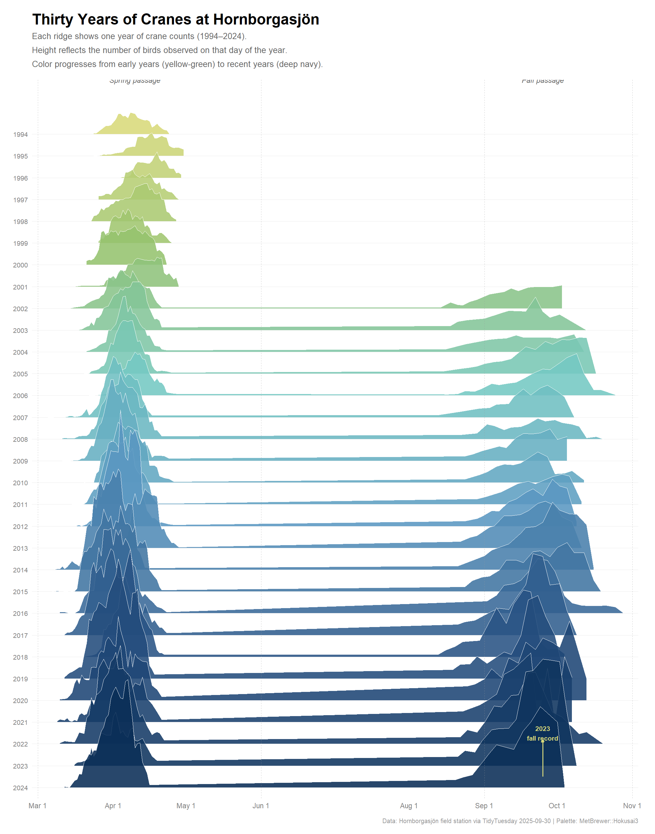
    title    = "Thirty Years of Cranes at Hornborgasjön",
    subtitle = "Each ridge shows one year of crane counts (1994–2024).\nHeight reflects the number of birds observed on that day of the year.\nColor progresses from early years (yellow-green) to recent years (deep navy).",
    x        = NULL,
    y        = NULL,
    caption  = "Data: Hornborgasjön field station via TidyTuesday 2025-09-30 | Palette: MetBrewer::Hokusai3"
  ) +
  ggplot2::theme_minimal(base_size = 11) +
  ggplot2::theme(
    plot.title         = ggplot2::element_text(size = 18, face = "bold", margin = ggplot2::margin(b = 6)),
    plot.subtitle      = ggplot2::element_text(size = 10, color = "grey40", lineheight = 1.4,
                                               margin = ggplot2::margin(b = 14)),
    plot.caption       = ggplot2::element_text(size = 7.5, color = "grey60", margin = ggplot2::margin(t = 10)),
    axis.text.x        = ggplot2::element_text(size = 8.5, color = "grey50"),
    axis.text.y        = ggplot2::element_text(size = 8, color = "grey50"),
    panel.grid.major.x = ggplot2::element_blank(),
    panel.grid.minor   = ggplot2::element_blank(),
    panel.grid.major.y = ggplot2::element_line(color = "grey92", linewidth = 0.3),
    legend.position    = "none",
    plot.background    = ggplot2::element_rect(fill = "white", color = NA),
    plot.margin        = ggplot2::margin(16, 20, 12, 16)
  )

p_ridge

# --- Secondary: Annual peak count trend ----------------------------------

p_line <- ggplot2::ggplot(annual_peaks_plot, ggplot2::aes(x = year, y = peak_count)) +
  ggplot2::geom_area(fill = "#5A97C1", alpha = 0.18) +
  ggplot2::geom_line(color = "#295384", linewidth = 0.9) +
  ggplot2::geom_point(
    ggplot2::aes(color = peak_month %in% c("Sep", "Oct")),
    size = 2.2
  ) +
  ggplot2::scale_color_manual(
    values = c(`FALSE` = "#295384", `TRUE` = "#D8D97A"),
    labels = c("Spring peak", "Fall peak"),
    name   = "Peak season"
  ) +
  ggrepel::geom_text_repel(
    ggplot2::aes(label = label),
    na.rm          = TRUE,
    size           = 3.0,
    color          = "grey30",
    lineheight     = 1.3,
    nudge_y        = 1800,
    segment.color  = "grey60",
    segment.size   = 0.3,
    box.padding    = 0.4,
    min.segment.length = 0
  ) +
  ggplot2::scale_x_continuous(breaks = seq(1994, 2024, by = 4)) +
  ggplot2::scale_y_continuous(
    labels = scales::comma,
    limits = c(0, 32000),
    expand = ggplot2::expansion(mult = c(0, 0.02))
  ) +
  ggplot2::labs(
    title    = "Annual Peak Crane Count, 1994–2024",
    subtitle = "Yellow dot marks the anomalous 2023 fall peak — the only non-spring record in 31 years",
    x        = NULL,
    y        = "Peak cranes observed",
    caption  = "Data: Hornborgasjön field station via TidyTuesday 2025-09-30"
  ) +
  ggplot2::theme_minimal(base_size = 11) +
  ggplot2::theme(
    plot.title         = ggplot2::element_text(size = 13, face = "bold"),
    plot.subtitle      = ggplot2::element_text(size = 9.5, color = "grey40"),
    plot.caption       = ggplot2::element_text(size = 7.5, color = "grey60"),
    panel.grid.minor   = ggplot2::element_blank(),
    panel.grid.major.x = ggplot2::element_blank(),
    legend.position    = "bottom",
    legend.title       = ggplot2::element_text(size = 8.5),
    legend.text        = ggplot2::element_text(size = 8),
    plot.background    = ggplot2::element_rect(fill = "white", color = NA),
    plot.margin        = ggplot2::margin(14, 20, 10, 16)
  )

p_line

Final thoughts and takeaways

The cranes of Hornborgasjön are a conservation success story written in daily counts. From a peak of fewer than 5,000 birds in 1994 — the first year after the lake’s restoration — the site grew to regularly host more than 20,000 cranes each spring by the 2010s, with the all-time spring record of 27,300 set in April 2019. Wetland restoration works, and these data make that visible with unusual precision.

Three findings deserve emphasis:

1. The growth is real and large. The fivefold increase over 30 years isn’t noise — it traces the expansion of the European crane population from near-collapse (the species was functionally extirpated from many parts of its range by the mid-20th century) to one of the continent’s most visible large-bird recovery stories. Hornborgasjön is both a beneficiary and a symbol of that turnaround.

2. The 2023 fall season was genuinely anomalous. Every year from 1994 through 2022 recorded its single-highest count during spring (March–May). In 2023, three consecutive observations in late September — September 18, 21, and 25 — all exceeded anything seen in that year’s spring and earned “Record observation” status from the field counters. Whether this reflects a true behavioral shift, a favorable autumn weather pattern that concentrated birds at the lake, or something else in the broader flyway isn’t answerable from this dataset alone, but it’s worth watching.

3. Spring phenology may be shifting. The peak-day data shows a subtle pattern: earlier years tended to peak in mid-April (day 100–110), while recent years more often peak in late March or early April (day 90–95). A handful of late-March peaks — 2016, 2017, 2018, 2019, 2022 — would have been exceptional a decade earlier. This is consistent with climate-driven earlier arrival documented for many European migratory species, though formal phenology analysis would require controlling for observer effort and weather.

The dataset’s limitation is also its strength: it’s a single fixed monitoring point, so changes in count reflect genuine changes in bird behavior and abundance rather than observer mobility. Thirty years is long enough to see slow trends; the field station’s continuity makes the comparison meaningful.

Tip

Data note: 161 observation records have missing counts (NA), nearly all due to canceled counts from bad weather or no-shows by the field crew. These were excluded from all summaries. They are genuinely absent observations, not zero-crane days — including them as zeroes would artificially depress the means.