Marking the FAO’s 80th anniversary with a deep dive into global food security indicators — tracking undernourishment, dietary adequacy, and food affordability across regions and time.
This dataset contains the FAO’s Suite of Food Security Indicators, compiled to commemorate the 80th anniversary of the Food and Agriculture Organization of the United Nations. The data captures various aspects of food insecurity through indicators selected by expert judgment, covering observations from 2005 onward.
Which indicators tend to vary together?
Do any indicators appear to be leading indicators of others?
How have confidence intervals changed over time or by region?
Loading necessary packages
My handy booster pack that allows me to install (if needed) and load my usual and favorite packages, as well as some helpful functions.
raw <- tidytuesdayR::tt_load('2025-10-14')food_security <- raw$food_security
Exploratory Data Analysis
The my_skim() function is a modified version of the skimr::skim() function that returns the number of missing data points (cells as NA) as well as the inverse (e.g.: number of rows that are notNA), the count, minimum, 25%, median, 75%, max, mean, geometric mean, and standard deviation. It also generates a little ASCII histogram. Neat!
# A tibble: 15 × 2
   Item                                                                        n
   <chr>                                                                   <int>
 1 Average dietary energy requirement (kcal/cap/day)                        4799
 2 Minimum dietary energy requirement  (kcal/cap/day)                       4799
 3 Gross domestic product per capita, PPP, (constant 2021 international $)  4662
 4 Number of people undernourished (million) (3-year average)               4482
 5 Prevalence of undernourishment (percent) (3-year average)                4482
 6 Number of women of reproductive age (15-49 years) affected by anemia (…  4446
 7 Prevalence of anemia among women of reproductive age (15-49 years) (pe…  4446
 8 Number of obese adults (18 years and older) (million)                    4310
 9 Prevalence of obesity in the adult population (18 years and older) (pe…  4310
10 Percentage of population using at least basic sanitation services (per…  4073
11 Dietary energy supply used in the estimation of the prevalence of unde…  4061
12 Incidence of caloric losses at retail distribution level (percent)       4059
13 Per capita food supply variability (kcal/cap/day)                        4055
14 Number of children under 5 years of age who are overweight (modeled es…  4042
15 Percentage of children under 5 years of age who are overweight (modell…  4042
food_security %>%count(Unit, sort =TRUE)
# A tibble: 8 × 2
  Unit           n
  <chr>      <int>
1 %          83111
2 million No 43069
3 kcal/cap/d 21520
4 g/cap/d    10722
5 Int$/cap    4662
6 index       3502
7 No          3182
8 km          1464
food_security %>%count(Flag, sort =TRUE)
# A tibble: 5 × 2
  Flag                                  n
  <chr>                             <int>
1 Estimated value                   90190
2 Figure from external organization 66447
3 Missing value                     10483
4 Missing value; suppressed          3766
5 Official figure                     346
# How many countries?n_distinct(food_security$Area)
[1] 249
Undernourishment and Food Affordability
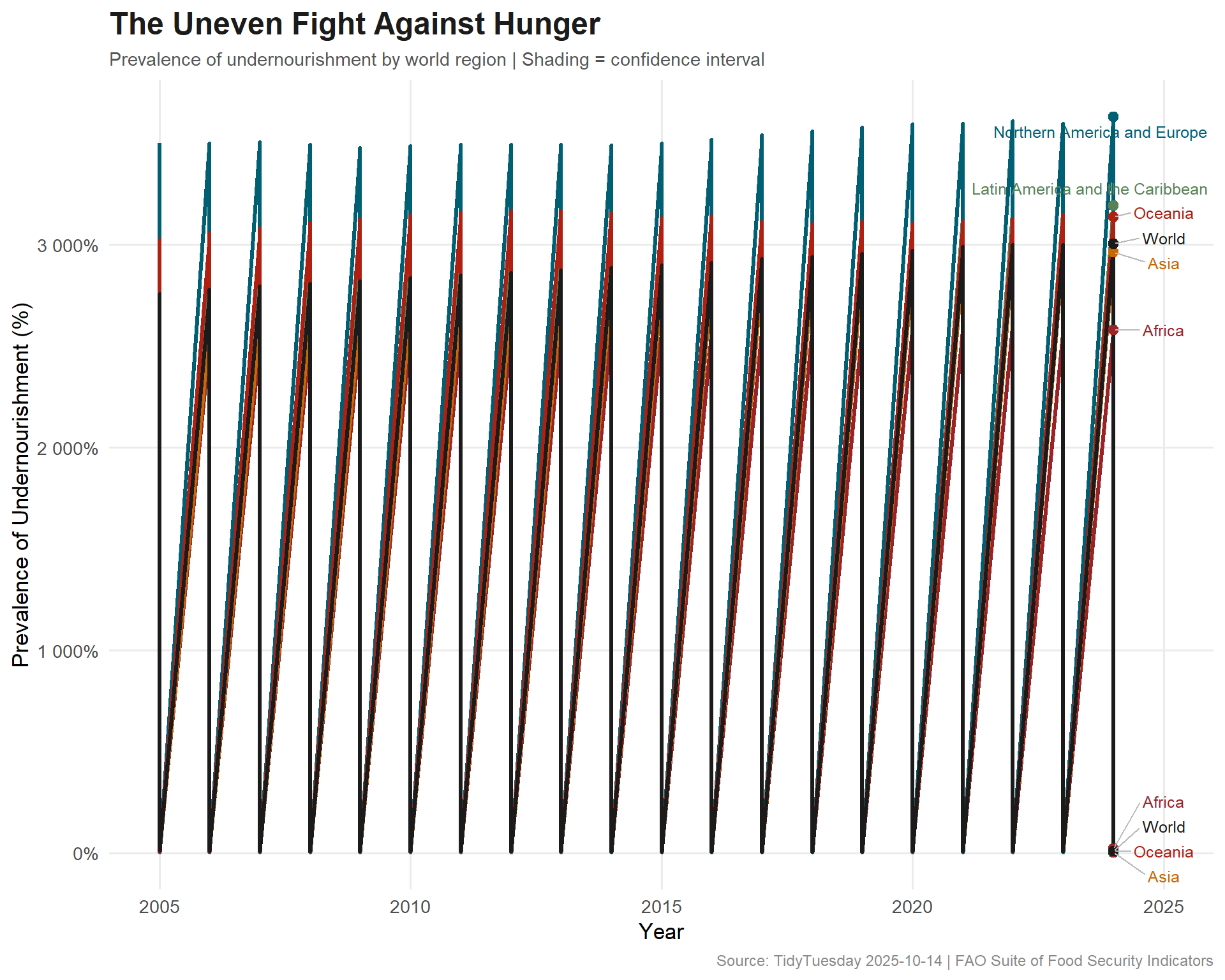
Prevalence of Undernourishment Over Time
undernourishment <- food_security %>%filter(str_detect(Item, regex("prevalence of undernourishment", ignore_case =TRUE))) %>%filter(!is.na(Value))# Global regions (filter out individual countries for trend)global_regions <-c("World", "Africa", "Asia", "Latin America and the Caribbean","Northern America and Europe", "Oceania")under_regions <- undernourishment %>%filter(Area %in% global_regions)under_regions %>%filter(Year_Start ==max(Year_Start)) %>%arrange(desc(Value))
# A tibble: 12 × 10
   Year_Start Year_End Area     Item  Unit   Value CI_Lower CI_Upper Flag  Note
        <dbl>    <dbl> <chr>    <chr> <chr>  <dbl>    <dbl>    <dbl> <chr> <chr>
 1       2024     2024 Norther… Diet… kcal… 3.63e3       NA       NA Esti… <NA>
 2       2024     2024 Latin A… Diet… kcal… 3.19e3       NA       NA Esti… <NA>
 3       2024     2024 Oceania  Diet… kcal… 3.14e3       NA       NA Esti… <NA>
 4       2024     2024 World    Diet… kcal… 3.01e3       NA       NA Esti… <NA>
 5       2024     2024 Asia     Diet… kcal… 2.96e3       NA       NA Esti… <NA>
 6       2024     2024 Africa   Diet… kcal… 2.58e3       NA       NA Esti… <NA>
 7       2024     2024 Africa   Prev… %     2.02e1       NA       NA Esti… <NA>
 8       2024     2024 World    Prev… %     8.2 e0       NA       NA Esti… <NA>
 9       2024     2024 Oceania  Prev… %     7.6 e0       NA       NA Esti… <NA>
10       2024     2024 Asia     Prev… %     6.7 e0       NA       NA Esti… <NA>
11       2024     2024 Latin A… Prev… %     5.1 e0       NA       NA Esti… <NA>
12       2024     2024 Norther… Prev… %     2.49e0       NA       NA Esti… <NA>
Dietary Energy Supply Adequacy
dietary_adequacy <- food_security %>%filter(str_detect(Item, regex("dietary energy supply adequacy", ignore_case =TRUE))) %>%filter(!is.na(Value), Area %in% global_regions)dietary_adequacy %>%filter(Year_Start ==max(Year_Start)) %>%arrange(Value)
# A tibble: 6 × 10
  Year_Start Year_End Area       Item  Unit  Value CI_Lower CI_Upper Flag  Note
       <dbl>    <dbl> <chr>      <chr> <chr> <dbl>    <dbl>    <dbl> <chr> <chr>
1       2022     2024 Africa     Aver… %       113       NA       NA Esti… <NA>
2       2022     2024 Asia       Aver… %       124       NA       NA Esti… <NA>
3       2022     2024 World      Aver… %       125       NA       NA Esti… <NA>
4       2022     2024 Oceania    Aver… %       127       NA       NA Esti… <NA>
5       2022     2024 Latin Ame… Aver… %       131       NA       NA Esti… <NA>
6       2022     2024 Northern … Aver… %       143       NA       NA Esti… <NA>
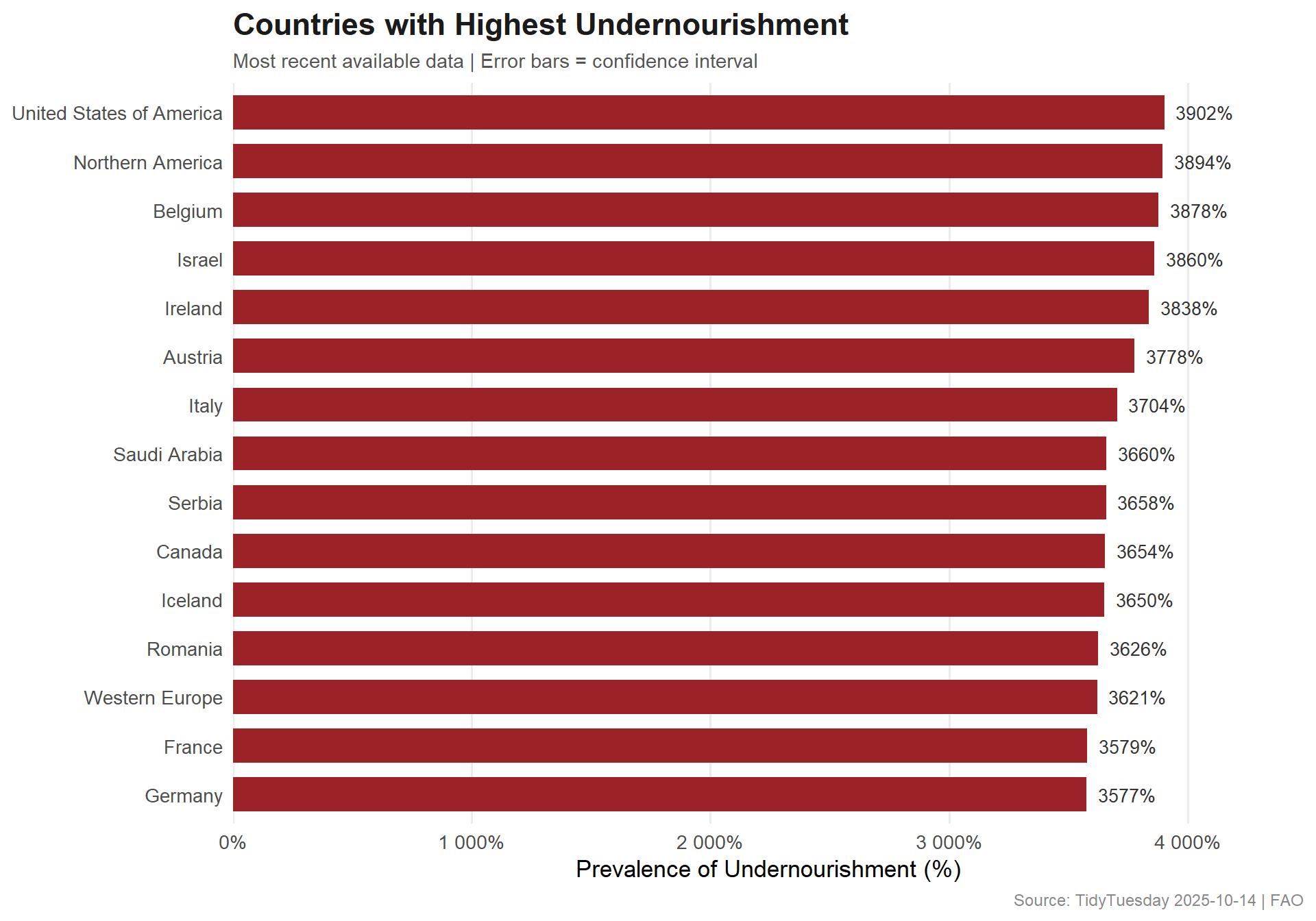
# A tibble: 15 × 6
   Area                     Year_Start Year_End Value CI_Lower CI_Upper
   <chr>                         <dbl>    <dbl> <dbl>    <dbl>    <dbl>
 1 United States of America       2023     2023  3902       NA       NA
 2 Northern America               2024     2024  3894       NA       NA
 3 Belgium                        2023     2023  3878       NA       NA
 4 Israel                         2023     2023  3860       NA       NA
 5 Ireland                        2023     2023  3838       NA       NA
 6 Austria                        2023     2023  3778       NA       NA
 7 Italy                          2023     2023  3704       NA       NA
 8 Saudi Arabia                   2023     2023  3660       NA       NA
 9 Serbia                         2023     2023  3658       NA       NA
10 Canada                         2023     2023  3654       NA       NA
11 Iceland                        2023     2023  3650       NA       NA
12 Romania                        2023     2023  3626       NA       NA
13 Western Europe                 2024     2024  3621       NA       NA
14 France                         2023     2023  3579       NA       NA
15 Germany                        2023     2023  3577       NA       NA
Visualizing Global Food Security
# Earth-tone palette for food/agricultureregion_cols <-c("World"="#1B1B1B","Africa"="#9B2226","Asia"="#CA6702","Latin America and the Caribbean"="#588157","Northern America and Europe"="#005F73","Oceania"="#AE2012")ggplot(under_regions, aes(x = Year_Start, y = Value, color = Area)) +geom_line(linewidth =1.1) +geom_point(data = under_regions %>%group_by(Area) %>%slice_max(Year_Start, n =1),size =2.5 ) +geom_ribbon(aes(ymin = CI_Lower, ymax = CI_Upper, fill = Area),alpha =0.1,color =NA ) +geom_text_repel(data = under_regions %>%group_by(Area) %>%slice_max(Year_Start, n =1),aes(label = Area),nudge_x =1,size =3.3,direction ="y",segment.color ="#BBBBBB" ) +scale_color_manual(values = region_cols) +scale_fill_manual(values = region_cols) +scale_y_continuous(labels = scales::percent_format(scale =1)) +labs(title ="The Uneven Fight Against Hunger",subtitle ="Prevalence of undernourishment by world region | Shading = confidence interval",x ="Year",y ="Prevalence of Undernourishment (%)",caption ="Source: TidyTuesday 2025-10-14 | FAO Suite of Food Security Indicators" ) +theme_minimal(base_size =13) +theme(plot.title =element_text(face ="bold", size =18, color ="#1B1B1B"),plot.subtitle =element_text(size =11, color ="#555555"),plot.caption =element_text(size =9, color ="#888888"),legend.position ="none",panel.grid.minor =element_blank() )
The FAO’s food security indicators paint a picture of progress interrupted. Global undernourishment declined steadily from the mid-2000s through 2015, but has since stalled or reversed in several regions — driven by conflict, climate shocks, and economic disruption (including the COVID-19 pandemic).
Africa remains the most food-insecure continent by a wide margin, with undernourishment prevalence far exceeding other regions. Asia has made remarkable progress in reducing hunger, but still carries the largest absolute number of undernourished people due to population size. The confidence intervals on these estimates are wide, reminding us that measuring hunger at a population level is inherently imprecise.
Important
Food security is not just about calories. The FAO framework captures multiple dimensions — availability, access, utilization, and stability. A country can have adequate caloric supply on paper while still having significant populations who can’t afford a nutritious diet. The “cost of a healthy diet” indicator is increasingly seen as a more meaningful measure than caloric adequacy alone.