This week we are exploring lead levels in water samples collected in Flint, Michigan in 2015. The data comes from a paper by Loux and Gibson (2018) who advocate for using this data as a teaching example in introductory statistics courses.
The Flint lead data provide a compelling example for introducing students to simple univariate descriptive statistics. In addition, they provide examples for discussion of sampling and data collection, as well as ethical data handling.
The data this week includes samples collected by the Michigan Department of Environment (MDEQ) and data from a citizen science project coordinated by Prof Marc Edwards and colleagues at Virginia Tech. Community-sourced samples were collected after concerns were raised about the MDEQ excluding samples from their data. You can read about the “murky” story behind this data here.
Thank you to @nzgwynn for submitting this dataset in #23!
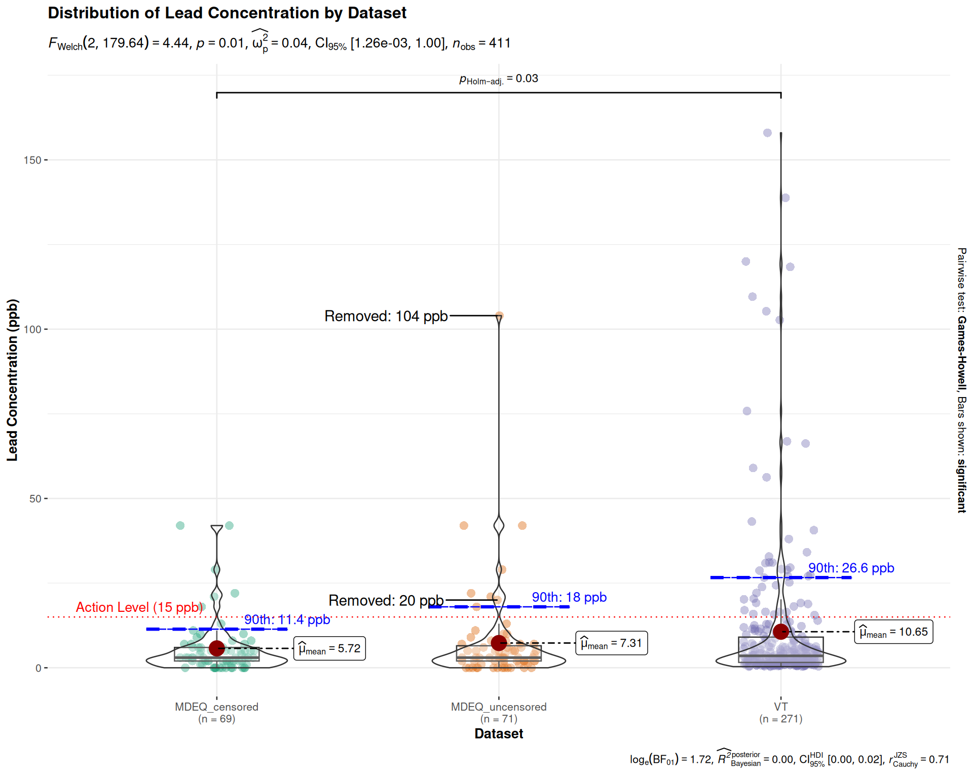
How does the distribution of lead levels differ between MDEQ and Virginia Tech datasets?
How do key statistics (mean, median, 90th percentile) change with/without excluded samples in the MDEQ sample?
Loading necessary packages
My handy booster pack that allows me to install (if needed) and load my usual and favorite packages, as well as some helpful functions.
Code
# Packages ----------------------------------------------------------------{# Install pak if it's not already installedif (!requireNamespace("pak", quietly =TRUE)) {install.packages("pak",repos =sprintf("https://r-lib.github.io/p/pak/stable/%s/%s/%s", .Platform$pkgType,R.Version()$os,R.Version()$arch ) ) }# CRAN Packages ---- install_booster_pack <-function(package, load =TRUE) {# Loop through each packagefor (pkg in package) {# Check if the package is installedif (!requireNamespace(pkg, quietly =TRUE)) {# If not installed, install the package pak::pkg_install(pkg) }# Load the packageif (load) {library(pkg, character.only =TRUE) } } }if (file.exists('packages.txt')) { packages <-read.table('packages.txt')install_booster_pack(package = packages$Package, load =FALSE)rm(packages) } else {## Packages ---- booster_pack <-c(### IO ----'fs','here','janitor','rio','tidyverse',# 'data.table',# 'mirai',# 'targets',# 'crew',### DB ----# 'arrow',# 'nanoparquet',# 'duckdb',# 'duckplyr',# 'dbplyr',### EDA ----'skimr',### Web ----# 'rvest',# 'polite',# 'plumber',# 'plumber2', #Still experimental# 'httr2',### Plot ----# 'paletteer',# 'ragg','camcorder','esquisse',# 'geofacet',# 'patchwork',# 'ggpubr', # Alternative to patchwork# 'marquee',# 'ggiraph',# 'geomtextpath',# 'ggpattern',# 'ggbump',# 'gghighlight',# 'ggdist',# 'ggforce',# 'gghalves',# 'ggtext',# 'ggrepel', # Suggested for non-overlapping labels# 'gganimate', # Suggested for animations# 'ggsignif',# 'ggTimeSeries',# 'tidyheatmaps',# 'ggdendro','ggstatsplot',### Modeling ----'tidymodels',### Shiny ----# 'shiny',# 'bslib',# 'DT',# 'plotly',### Reporting ----# 'quarto','gt','gtsummary',### Spatial ----# 'sf',# 'geoarrow',# 'duckdbfs',# 'duckspatial',# 'ducksf',# 'tidycensus', # Needs API# 'mapgl',# 'dataRetrieval', # Needs API# 'StreamCatTools',### Misc ----'tidytuesdayR'# 'devtools',# 'usethis',# 'remotes' )# ! Change load flag to load packagesinstall_booster_pack(package = booster_pack, load =TRUE)rm(install_booster_pack, booster_pack) }# GitHub Packages ----# github_packages <- c(# "seanthimons/ComptoxR"# )# # Ensure remotes is installed# if (!requireNamespace("remotes", quietly = TRUE)) {# install.packages("remotes")# }# # Loop through each GitHub package# for (pkg in github_packages) {# # Extract package name from the "user/repo" string# pkg_name <- sub(".*/", "", pkg)# # Check if the package is installed# if (!requireNamespace(pkg_name, quietly = TRUE)) {# # If not installed, install the latest release from GitHub# remotes::install_github(paste0(pkg, "@*release"))# }# # Load the package# library(pkg_name, character.only = TRUE)# }# rm(github_packages, pkg, pkg_name)# Custom Functions ----`%ni%`<-Negate(`%in%`) geometric_mean <-function(x) {exp(mean(log(x[x >0]), na.rm =TRUE)) } my_skim <-skim_with(numeric =sfl(n = length,min =~min(.x, na.rm = T),p25 =~ stats::quantile(., probs = .25, na.rm =TRUE, names =FALSE),med =~median(.x, na.rm = T),p75 =~ stats::quantile(., probs = .75, na.rm =TRUE, names =FALSE),max =~max(.x, na.rm = T),mean =~mean(.x, na.rm = T),geo_mean =~geometric_mean(.x),sd =~ stats::sd(., na.rm =TRUE),hist =~inline_hist(., 5) ),append =FALSE )}
Load raw data from package
raw <- tidytuesdayR::tt_load('2025-11-04')flint_mdeq <- raw$flint_mdeqflint_vt <- raw$flint_vt
Exploratory Data Analysis
The my_skim() function is a modified version of the skimr::skim() function that returns the number of missing data points (cells as NA) as well as the inverse (e.g.: number of rows that are notNA), the count, minimum, 25%, median, 75%, max, mean, geometric mean, and standard deviation. It also generates a little ASCII histogram. Neat!
MDEQ data
I also remove the sample and notes column since I am just interested in the numerical data.
This also helps us examine the second proposed question from the repo.
At the crux of this exercise is reproducing the determination if the samples collected by MDEQ with and without censoring of the data would cause a violation of existing state and federal law for lead contamination. For lead, the actionable level is 15 parts-per-billion (ppb).
# Combine the three datasets into one tidy dataframecombined_data <-bind_rows( flint_mdeq %>%mutate(dataset ="MDEQ_uncensored", lead = lead, .keep ='none'), flint_mdeq %>%mutate(dataset ="MDEQ_censored", lead = lead2, .keep ='none'), flint_vt %>%mutate(dataset ="VT", lead = lead, .keep ='none')) %>%filter(!is.na(lead)) # Remove NA values from the censored dataset# New skim functionlead_skim <-skim_with(numeric =sfl(n = length,p90 =~ stats::quantile(., probs = .9, na.rm =TRUE, names =FALSE),max =~max(.x, na.rm = T) ),append =FALSE)# Running the new skim function that finds the 90th percentile to see if there was an exceedencecombined_data %>%group_by(dataset) %>%lead_skim()
Data summary
Name
Piped data
Number of rows
411
Number of columns
2
_______________________
Column type frequency:
numeric
1
________________________
Group variables
dataset
Variable type: numeric
skim_variable
dataset
n_missing
complete_rate
n
p90
max
lead
MDEQ_censored
0
1
69
11.40
42
lead
MDEQ_uncensored
0
1
71
18.00
104
lead
VT
0
1
271
26.64
158
Here, we see that at the 90th percentile for the samples collected by MDEQ within the censored dataset it appears to pass (11.4 ppb), requiring no end-user notification or action. However, with the uncensored dataset, the 90th percentile becomes 18.0 ppb.
Important
It should be noted that the public health goal for lead is 0.00 ppb, as there is no safe amount of lead exposure.
If we want to see if multiple datasets are different from each other, we can run some simple statistical tests. As you requested, we’ll use an Analysis of Variance (ANOVA) test. This test will help us determine if there are any statistically significant differences between the means of our three groups:
The uncensored Michigan Department of Environment (MDEQ) data.
The “censored” MDEQ data (with two high-value samples removed).
The Virginia Tech (VT) citizen-collected data.
We will use the tidymodels framework to set up and run the ANOVA.
# Define the model specification using tidymodelslm_spec <-linear_reg() %>%set_engine("lm")# Define the recipeanova_recipe <-recipe(lead ~ dataset, data = combined_data)# Create the workflowanova_workflow <-workflow() %>%add_model(lm_spec) %>%add_recipe(anova_recipe)# Fit the workflow and extract the resultsanova_fit <-fit(anova_workflow, data = combined_data)# Get the overall ANOVA table by extracting the engine fitanova(extract_fit_engine(anova_fit))
Analysis of Variance Table

Response: ..y
           Df Sum Sq Mean Sq F value  Pr(>F)
dataset     2   1653  826.45  2.3311 0.09848 .
Residuals 408 144649  354.53
---
Signif. codes:  0 '***' 0.001 '**' 0.01 '*' 0.05 '.' 0.1 ' ' 1
# Tidy the results to get the model coefficientsbroom::tidy(anova_fit)
Before we plot any data, we’ll set up a camcorder session to capture our plot(s) at the proper resolution. Not always needed, but helpful for iterating when making complex plots.
Warning in gg_record(here::here("posts", "2025-11-04", "output"), device =
"png", : Writing to a folder that already exists. gg_playback may use more
files than intended!
The very small p-value (p.value < 0.05) for the dataset term indicates that there is a statistically significant difference between the mean lead levels of at least two of the groups.
To get a more intuitive visualization and a comprehensive statistical summary in one go, we can use the ggbetweenstats() function from the ggstatsplot package. This will create a plot and run the appropriate statistical tests automatically.
# Calculate 90th percentile for each datasetp90_data <- combined_data %>%group_by(dataset) %>%summarize(p90 =quantile(lead, probs =0.9, na.rm =TRUE))ggbetweenstats(data = combined_data,x = dataset,y = lead,title ="Distribution of Lead Concentration by Dataset",xlab ="Dataset",ylab ="Lead Concentration (ppb)",messages =FALSE) +# Add 90th percentile lines for each datasetgeom_crossbar(data = p90_data,aes(x = dataset, y = p90, ymin = p90, ymax = p90),width =0.5,color ="blue",linetype ="dashed" ) +geom_text(data = p90_data,aes(x = dataset, y = p90, label =paste("90th:", round(p90, 1), 'ppb')),vjust =-0.5,color ="blue",nudge_x =0.25 ) +# Add layers to the ggplot objectgeom_hline(yintercept =15,linetype ="dotted",color ="red" ) +annotate("text",x =0.5,y =15,label ="Action Level (15 ppb)",vjust =-0.5,color ="red",hjust =0 ) + ggrepel::geom_text_repel(data = . %>% dplyr::filter(dataset =="MDEQ_uncensored", lead %in%c(20, 104)),aes(label =paste("Removed:", lead, "ppb")),nudge_x =-0.4,min.segment.length =0 )
Final thoughts and takeaways
The Flint water crisis was an avoidable tragedy born from a series of deliberate decisions that prioritized cost-saving measures over public health. The catastrophe was not the result of a natural disaster or unforeseeable accident, but a direct consequence of switching the city’s water source to the corrosive Flint River without implementing the necessary anti-corrosion treatments. This critical and well-understood water treatment step, which would have cost approximately $140 a day, was skipped, allowing lead from aging pipes to leach into the drinking water. The crisis was further compounded by a systemic failure of oversight and a dismissal of residents’ early complaints about the water’s quality, making this a man-made disaster that could have been entirely averted with responsible governance and adherence to established public health standards.
The long-term health consequences for Flint’s residents, particularly its children, are still unfolding. Exposure to high levels of lead has left a legacy of potential developmental delays, learning disabilities, and behavioral issues that will require sustained support for years to come. Studies have also pointed to a spike in both physical and mental health problems among residents, including skin rashes, hair loss, anxiety, and depression in the wake of the crisis.