Tidy Tuesday: WHO TB Burden Data

tidytuesday

public-health

epidemiology

Tracking the global tuberculosis burden through WHO data — which regions carry the heaviest load, how has mortality shifted over time, and what role does HIV co-infection play?

Author

Sean Thimons

Published

November 11, 2025

Preface

From TidyTuesday repository.

Global tuberculosis burden estimates from the World Health Organization, curated via the getTBinR R package. Tuberculosis remains one of the world’s deadliest infectious diseases — WHO estimates that 10.6 million people fell ill with TB in 2021, and 1.6 million died from the disease.

Are there years showing unusual TB metric spikes or drops globally?

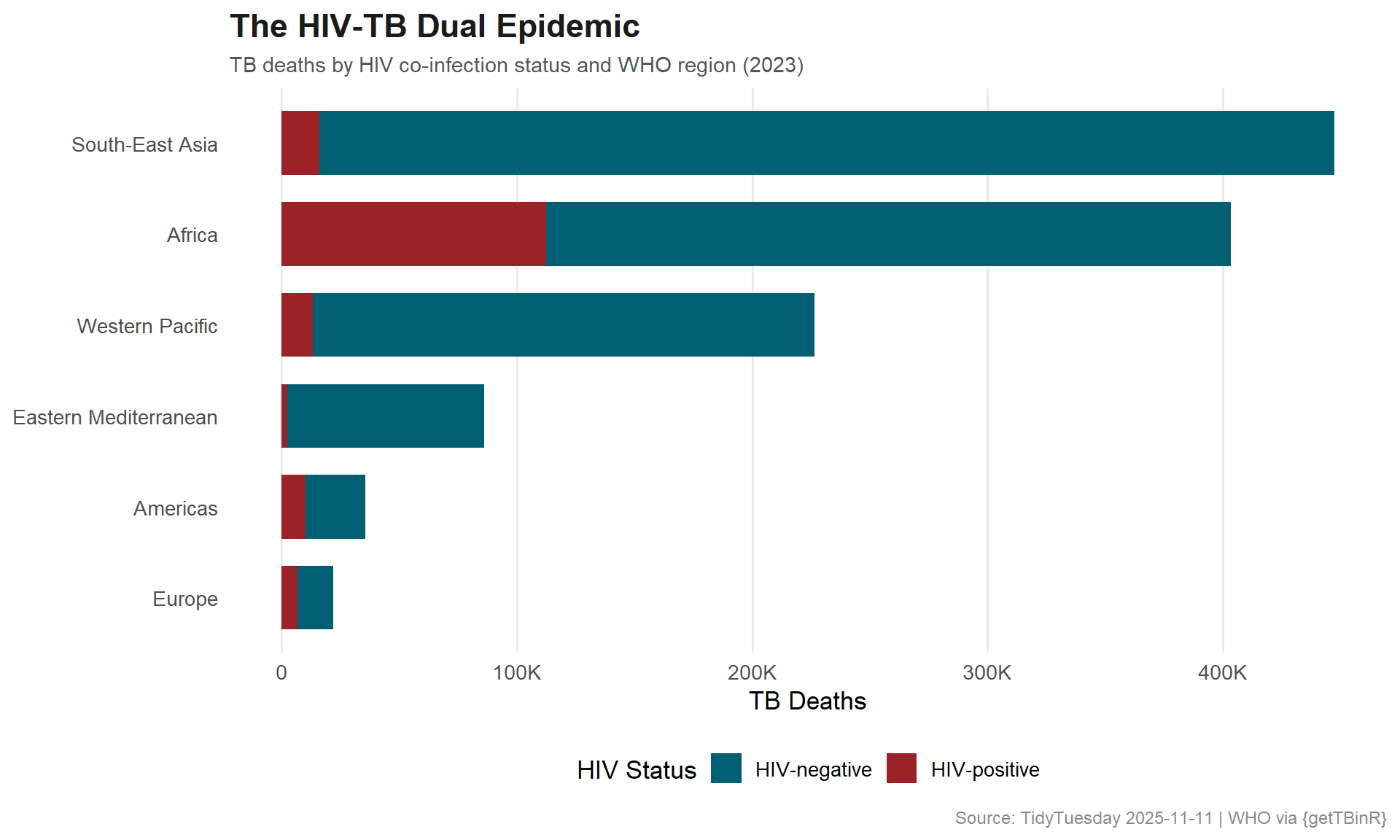
How does TB mortality differ between HIV-positive and HIV-negative populations?

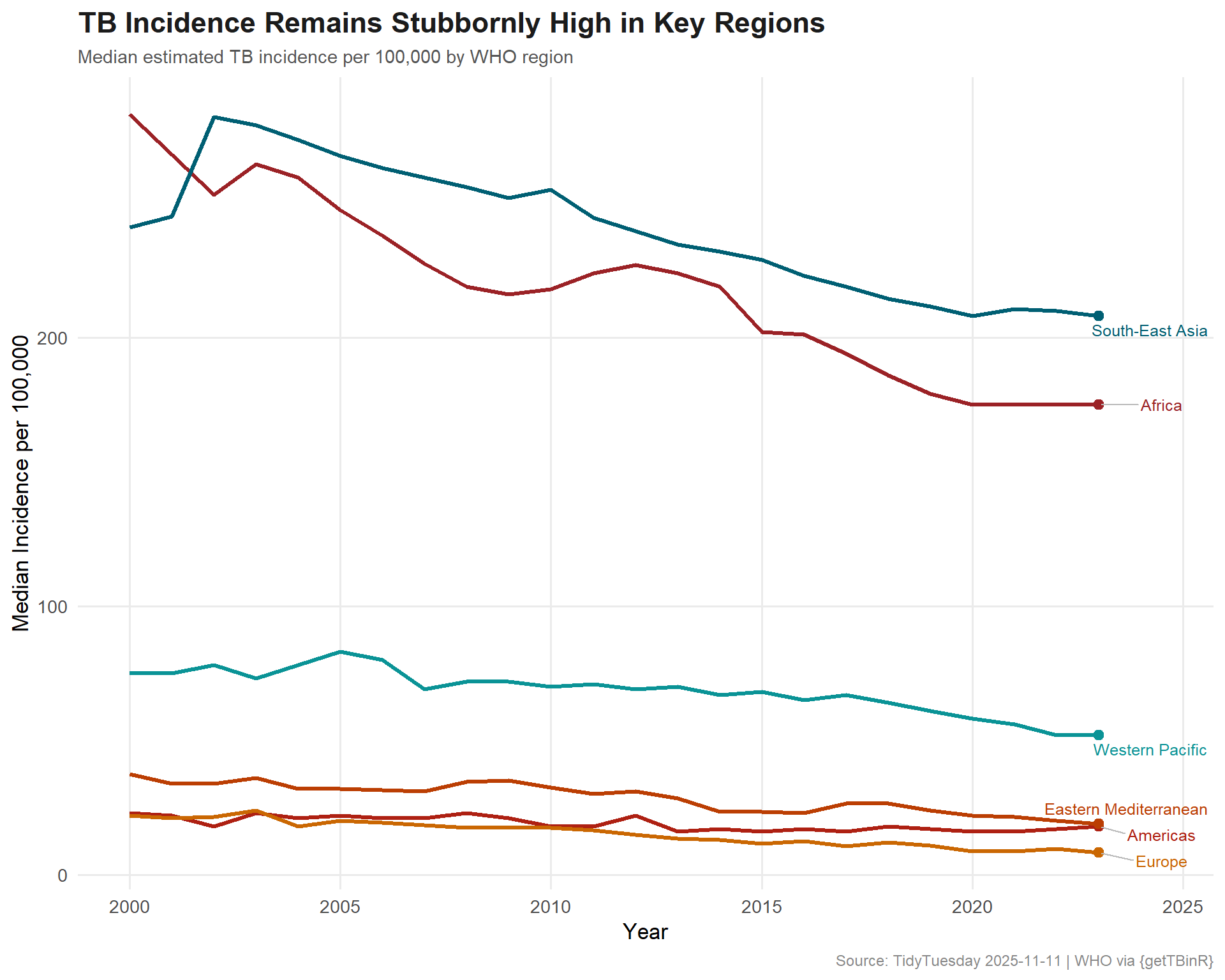
Which regions demonstrate consistently high TB burden across multiple years?

Loading necessary packages

My handy booster pack that allows me to install (if needed) and load my usual and favorite packages, as well as some helpful functions.

Code

# Packages ----------------------------------------------------------------

{
  if (!requireNamespace("pak", quietly = TRUE)) {
    install.packages(
      "pak",
      repos = sprintf(
        "https://r-lib.github.io/p/pak/stable/%s/%s/%s",
        .Platform$pkgType,
        R.Version()$os,
        R.Version()$arch
      )
    )
  }

  install_booster_pack <- function(package, load = TRUE) {
    for (pkg in package) {
      if (!requireNamespace(pkg, quietly = TRUE)) {
        pak::pkg_install(pkg)
      }
      if (load) {
        library(pkg, character.only = TRUE)
      }
    }
  }

  if (file.exists('packages.txt')) {
    packages <- read.table('packages.txt')
    install_booster_pack(package = packages$Package, load = FALSE)
    rm(packages)
  } else {
    booster_pack <- c(
      ### IO ----
      'fs',
      'here',
      'janitor',
      'rio',
      'tidyverse',

      ### EDA ----
      'skimr',

      ### Plot ----
      'ggrepel',
      'ggtext',
      'scales',

      ### Misc ----
      'tidytuesdayR'
    )

    install_booster_pack(package = booster_pack, load = TRUE)
    rm(install_booster_pack, booster_pack)
  }

  # Custom Functions ----

  `%ni%` <- Negate(`%in%`)

  geometric_mean <- function(x) {
    exp(mean(log(x[x > 0]), na.rm = TRUE))
  }

  my_skim <- skim_with(
    numeric = sfl(
      n = length,
      min = ~ min(.x, na.rm = T),
      p25 = ~ stats::quantile(., probs = .25, na.rm = TRUE, names = FALSE),
      med = ~ median(.x, na.rm = T),
      p75 = ~ stats::quantile(., probs = .75, na.rm = TRUE, names = FALSE),
      max = ~ max(.x, na.rm = T),
      mean = ~ mean(.x, na.rm = T),
      geo_mean = ~ geometric_mean(.x),
      sd = ~ stats::sd(., na.rm = TRUE),
      hist = ~ inline_hist(., 5)
    ),
    append = FALSE
  )
}

Load raw data from package

raw <- tidytuesdayR::tt_load('2025-11-11')

tb <- raw$who_tb_data

Exploratory Data Analysis

The my_skim() function is a modified version of the skimr::skim() function that returns the number of missing data points (cells as NA) as well as the inverse (e.g.: number of rows that are not NA), the count, minimum, 25%, median, 75%, max, mean, geometric mean, and standard deviation. It also generates a little ASCII histogram. Neat!

TB Burden

tb %>%
  my_skim(.)

Data summary
Name	Piped data
Number of rows	5117
Number of columns	18
_______________________
Column type frequency:
character	4
numeric	14
________________________
Group variables	None

Variable type: character

skim_variable	complete_rate	min	max	n_unique
country	1	4	56	215
g_whoregion	1	6	21	6
iso2	1	2	4	215
iso3	1	3	3	215

Variable type: numeric

skim_variable	n_missing	complete_rate	n	min	p25	med	p75	max	mean	geo_mean	sd	hist
iso_numeric	0	1.00	5117	4	212.00	430.00	646.00	894	431.79	315.72	253.11	▇▇▇▇▆
year	0	1.00	5117	2000	2006.00	2012.00	2018.00	2023	2011.56	2011.55	6.91	▇▇▆▇▇
c_cdr	293	0.94	5117	0	60.00	80.00	87.00	240	73.36	70.45	19.44	▁▇▁▁▁
c_newinc_100k	185	0.96	5117	0	10.00	36.00	95.00	947	73.33	33.09	104.03	▇▁▁▁▁
cfr	128	0.97	5117	0	0.08	0.11	0.22	1	0.16	0.12	0.13	▇▂▁▁▁
e_inc_100k	0	1.00	5117	0	12.00	46.00	160.00	1590	122.49	45.27	183.69	▇▁▁▁▁
e_inc_num	0	1.00	5117	0	210.00	2900.00	17000.00	3590000	52027.21	1973.33	250579.80	▇▁▁▁▁
e_mort_100k	24	1.00	5117	0	0.96	4.50	23.00	533	25.44	5.27	53.26	▇▁▁▁▁
e_mort_exc_tbhiv_100k	24	1.00	5117	0	0.85	3.80	19.00	188	14.44	4.14	22.34	▇▁▁▁▁
e_mort_exc_tbhiv_num	24	1.00	5117	0	15.00	210.00	1700.00	786000	6631.70	230.91	37001.66	▇▁▁▁▁
e_mort_num	24	1.00	5117	0	18.00	260.00	2800.00	979000	8975.11	294.52	45867.33	▇▁▁▁▁
e_mort_tbhiv_100k	24	1.00	5117	0	0.01	0.19	2.20	481	10.95	0.69	38.68	▇▁▁▁▁
e_mort_tbhiv_num	24	1.00	5117	0	0.00	16.00	340.00	223000	2333.54	92.96	12056.61	▇▁▁▁▁
e_pop_num	0	1.00	5117	1552	762582.00	5939341.00	21547461.00	1438069593	33406512.96	3624185.87	131759733.15	▇▁▁▁▁

tb %>%
  dplyr::count(g_whoregion, sort = TRUE)

# A tibble: 6 × 2
  g_whoregion               n
  <chr>                 <int>
1 Europe                 1286
2 Africa                 1117
3 Americas               1060
4 Western Pacific         888
5 Eastern Mediterranean   528
6 South-East Asia         238

tb %>%
  summarize(
    min_year = min(year),
    max_year = max(year),
    n_countries = n_distinct(country)
  )

# A tibble: 1 × 3
  min_year max_year n_countries
     <dbl>    <dbl>       <int>
1     2000     2023         215

Regional TB Burden Over Time

Incidence Trends by WHO Region

regional_trend <- tb %>%
  filter(!is.na(e_inc_100k)) %>%
  group_by(g_whoregion, year) %>%
  summarize(
    median_incidence = median(e_inc_100k, na.rm = TRUE),
    total_cases = sum(e_inc_num, na.rm = TRUE),
    .groups = "drop"
  )

regional_trend %>%
  filter(year == max(year)) %>%
  arrange(desc(median_incidence))

# A tibble: 6 × 4
  g_whoregion            year median_incidence total_cases
  <chr>                 <dbl>            <dbl>       <dbl>
1 South-East Asia        2023           208        3819410
2 Africa                 2023           175        2553296
3 Western Pacific        2023            52        2968369
4 Eastern Mediterranean  2023            19         936694
5 Americas               2023            18         342030
6 Europe                 2023             8.25      224611

HIV-TB Co-infection: Mortality Breakdown

hiv_tb <- tb %>%
  filter(!is.na(e_mort_tbhiv_100k), !is.na(e_mort_exc_tbhiv_100k)) %>%
  group_by(g_whoregion, year) %>%
  summarize(
    mort_hiv_pos = sum(e_mort_tbhiv_num, na.rm = TRUE),
    mort_hiv_neg = sum(e_mort_exc_tbhiv_num, na.rm = TRUE),
    total_mort = sum(e_mort_num, na.rm = TRUE),
    .groups = "drop"
  ) %>%
  mutate(pct_hiv = mort_hiv_pos / total_mort)

hiv_tb %>%
  filter(year == max(year)) %>%
  arrange(desc(pct_hiv))

# A tibble: 6 × 6
  g_whoregion            year mort_hiv_pos mort_hiv_neg total_mort pct_hiv
  <chr>                 <dbl>        <dbl>        <dbl>      <dbl>   <dbl>
1 Europe                 2023         6535        15477      22482  0.291 
2 Americas               2023        10018        25361      35504  0.282 
3 Africa                 2023       112253       291344     402805  0.279 
4 Western Pacific        2023        13127       213261     225208  0.0583
5 South-East Asia        2023        15909       431578     446608  0.0356
6 Eastern Mediterranean  2023         2202        83812      86254  0.0255

Important

In the African region, HIV-associated TB mortality accounts for a substantial share of all TB deaths — a dual epidemic that demands integrated treatment programs addressing both diseases simultaneously.

Top Burden Countries

latest_year <- max(tb$year, na.rm = TRUE)

top_burden <- tb %>%
  filter(year == latest_year, !is.na(e_inc_num)) %>%
  arrange(desc(e_inc_num)) %>%
  head(10) %>%
  select(country, g_whoregion, e_inc_num, e_inc_100k, e_mort_100k, c_cdr)

top_burden

# A tibble: 10 × 6
   country                    g_whoregion e_inc_num e_inc_100k e_mort_100k c_cdr
   <chr>                      <chr>           <dbl>      <dbl>       <dbl> <dbl>
 1 India                      South-East…   2800000        195        22      85
 2 Indonesia                  Western Pa…   1090000        387        47      74
 3 China                      Western Pa…    741000         52         1.9    76
 4 Philippines                Western Pa…    739000        643        32      78
 5 Pakistan                   Eastern Me…    686000        277        20      69
 6 Nigeria                    Africa         499000        219        31      74
 7 Bangladesh                 South-East…    379000        221        26      80
 8 Democratic Republic of th… Africa         334000        316        41      77
 9 Myanmar                    South-East…    302000        558        90      43
10 South Africa               Africa         270000        427        88      79

Visualizing the Global TB Burden

# Public health palette — clinical but human
region_cols <- c(
  "#9B2226",  # deep red
  "#AE2012",  # rust
  "#BB3E03",  # dark orange
  "#CA6702",  # amber
  "#005F73",  # deep teal
  "#0A9396"   # teal
)

ggplot(regional_trend, aes(x = year, y = median_incidence, color = g_whoregion)) +
  geom_line(linewidth = 1.1) +
  geom_point(
    data = regional_trend %>%
      group_by(g_whoregion) %>%
      slice_max(year, n = 1),
    size = 2.5
  ) +
  geom_text_repel(
    data = regional_trend %>%
      group_by(g_whoregion) %>%
      slice_max(year, n = 1),
    aes(label = g_whoregion),
    nudge_x = 1.5,
    size = 3.3,
    direction = "y",
    segment.color = "#BBBBBB"
  ) +
  scale_color_manual(values = region_cols) +
  scale_y_continuous(labels = scales::comma) +
  labs(
    title = "TB Incidence Remains Stubbornly High in Key Regions",
    subtitle = "Median estimated TB incidence per 100,000 by WHO region",
    x = "Year",
    y = "Median Incidence per 100,000",
    caption = "Source: TidyTuesday 2025-11-11 | WHO via {getTBinR}"
  ) +
  theme_minimal(base_size = 13) +
  theme(
    plot.title = element_text(face = "bold", size = 17, color = "#1B1B1B"),
    plot.subtitle = element_text(size = 11, color = "#555555"),
    plot.caption = element_text(size = 9, color = "#888888"),
    legend.position = "none",
    panel.grid.minor = element_blank()
  )

hiv_long <- hiv_tb %>%
  select(g_whoregion, year, mort_hiv_pos, mort_hiv_neg) %>%
  pivot_longer(
    cols = starts_with("mort_"),
    names_to = "hiv_status",
    values_to = "deaths"
  ) %>%
  mutate(
    hiv_label = ifelse(hiv_status == "mort_hiv_pos", "HIV-positive", "HIV-negative")
  )

# Focus on latest year
hiv_latest <- hiv_long %>%
  filter(year == max(year)) %>%
  group_by(g_whoregion) %>%
  mutate(total = sum(deaths), pct = deaths / total) %>%
  ungroup() %>%
  mutate(g_whoregion = fct_reorder(g_whoregion, total))

hiv_cols <- c("HIV-positive" = "#9B2226", "HIV-negative" = "#005F73")

ggplot(hiv_latest, aes(x = g_whoregion, y = deaths, fill = hiv_label)) +
  geom_col(width = 0.7) +
  scale_y_continuous(labels = scales::label_number(scale_cut = scales::cut_short_scale())) +
  scale_fill_manual(values = hiv_cols, name = "HIV Status") +
  coord_flip() +
  labs(
    title = "The HIV-TB Dual Epidemic",
    subtitle = paste0("TB deaths by HIV co-infection status and WHO region (", max(hiv_tb$year), ")"),
    x = NULL,
    y = "TB Deaths",
    caption = "Source: TidyTuesday 2025-11-11 | WHO via {getTBinR}"
  ) +
  theme_minimal(base_size = 13) +
  theme(
    plot.title = element_text(face = "bold", size = 17, color = "#1B1B1B"),
    plot.subtitle = element_text(size = 11, color = "#555555"),
    plot.caption = element_text(size = 9, color = "#888888"),
    legend.position = "bottom",
    panel.grid.major.y = element_blank(),
    panel.grid.minor = element_blank()
  )

Final thoughts and takeaways

Tuberculosis is a disease of inequality. The data shows that TB burden clusters overwhelmingly in the South-East Asia and African regions, where poverty, overcrowding, and weak health systems create perfect conditions for transmission. Despite being both preventable and curable, TB kills more than 1.5 million people annually — making it the world’s deadliest infectious disease alongside COVID-19.

The HIV-TB co-infection story is particularly stark in sub-Saharan Africa, where the two epidemics feed on each other. HIV weakens the immune system, making TB infection more likely to progress to active disease. TB, in turn, accelerates HIV progression. Integrated treatment programs that address both diseases simultaneously have been a critical public health innovation.

Tip

The case detection rate (c_cdr) is a crucial indicator that often gets overlooked. A country can have high incidence but low detection — meaning people are getting sick but not being diagnosed or treated. This “missing” TB is both a humanitarian crisis and an ongoing transmission risk.