A text analysis of the complete Sherlock Holmes canon — exploring sentence patterns, story lengths, and the linguistic fingerprints that distinguish Watson’s narration from Holmes’s dialogue.
This collection contains the full line-by-line text of Sir Arthur Conan Doyle’s Sherlock Holmes stories and novels, organized by book and line number. The dataset is sourced from the sherlock R package by Emil Hvitfeldt and is designed for stylometric analysis, sentiment examination, and literary exploration.
How do Watson’s narration patterns differ from Holmes’s speech patterns?
What variations exist in sentence length across different stories?
Does tone shift when comparing Watson’s narration to Holmes’s direct dialogue?
Loading necessary packages
My handy booster pack that allows me to install (if needed) and load my usual and favorite packages, as well as some helpful functions.
raw <- tidytuesdayR::tt_load('2025-11-18')holmes <- raw$holmes
Exploratory Data Analysis
The my_skim() function is a modified version of the skimr::skim() function that returns the number of missing data points (cells as NA) as well as the inverse (e.g.: number of rows that are notNA), the count, minimum, 25%, median, 75%, max, mean, geometric mean, and standard deviation. It also generates a little ASCII histogram. Neat!
Sherlock Holmes Text
holmes %>%filter(!is.na(text), text !="") %>%mutate(n_chars =nchar(text)) %>%my_skim(.)
Data summary
Name
Piped data
Number of rows
52610
Number of columns
4
_______________________
Column type frequency:
character
2
numeric
2
________________________
Group variables
None
Variable type: character
skim_variable
n_missing
complete_rate
min
max
empty
n_unique
whitespace
book
0
1
12
43
0
48
0
text
0
1
2
69
0
51915
0
Variable type: numeric
skim_variable
n_missing
complete_rate
n
min
p25
med
p75
max
mean
geo_mean
sd
hist
line_num
0
1
52610
1
341
688
1711.75
6969
1393.15
682.28
1653.39
▇▁▁▁▁
n_chars
0
1
52610
2
60
66
68.00
69
57.90
53.03
17.03
▁▁▁▁▇
book_lengths <- holmes %>%filter(!is.na(text), text !="") %>%count(book, sort =TRUE, name ="n_lines")book_lengths
# A tibble: 48 × 2
   book                                        n_lines
   <chr>                                         <int>
 1 The Hound of the Baskervilles                  5468
 2 The Valley Of Fear                             5373
 3 A Study In Scarlet                             3945
 4 The Sign of the Four                           3817
 5 The Naval Treaty                               1192
 6 The Adventure of the Priory School             1095
 7 The Adventure of Wisteria Lodge                1046
 8 The Adventure of the Bruce-Partington Plans    1024
 9 The Adventure of the Second Stain               917
10 The Adventure of the Devil's Foot               899
# ℹ 38 more rows
Text Analysis
Tokenization and Word Frequencies
holmes_words <- holmes %>%filter(!is.na(text), text !="") %>%unnest_tokens(word, text) %>%anti_join(stop_words, by ="word")# Top words across entire canonholmes_words %>%count(word, sort =TRUE) %>%head(20)
# A tibble: 20 × 2
   word        n
   <chr>   <int>
 1 holmes   2403
 2 time      879
 3 sir       846
 4 watson    809
 5 house     773
 6 night     718
 7 door      687
 8 hand      649
 9 found     570
10 eyes      553
11 left      538
12 heard     519
13 day       510
14 matter    485
15 morning   467
16 cried     454
17 round     444
18 friend    433
19 window    425
20 head      394
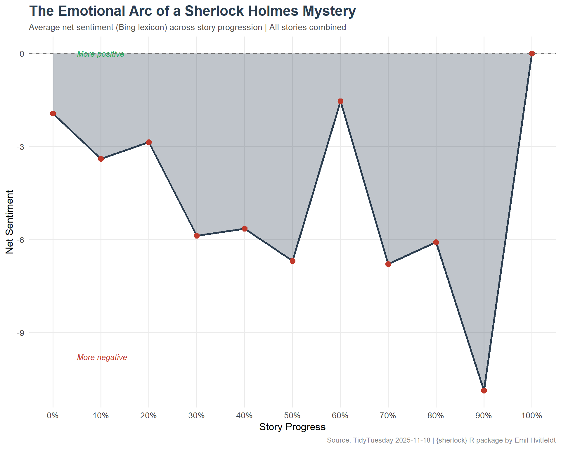
Sentiment Arc Across Stories
How does sentiment evolve through a typical Holmes story?
# Use Bing lexicon for positive/negativesentiment_by_line <- holmes %>%filter(!is.na(text), text !="") %>%group_by(book) %>%mutate(line_pct = line_num /max(line_num, na.rm =TRUE)) %>%ungroup() %>%unnest_tokens(word, text) %>%inner_join(get_sentiments("bing"), by ="word") %>%mutate(score =ifelse(sentiment =="positive", 1, -1))# Aggregate by book and story progress (deciles)arc_data <- sentiment_by_line %>%mutate(decile =floor(line_pct *10) /10) %>%group_by(book, decile) %>%summarize(net_sentiment =sum(score),.groups ="drop" )# Average arc across all booksavg_arc <- arc_data %>%group_by(decile) %>%summarize(mean_sentiment =mean(net_sentiment, na.rm =TRUE),.groups ="drop" )avg_arc
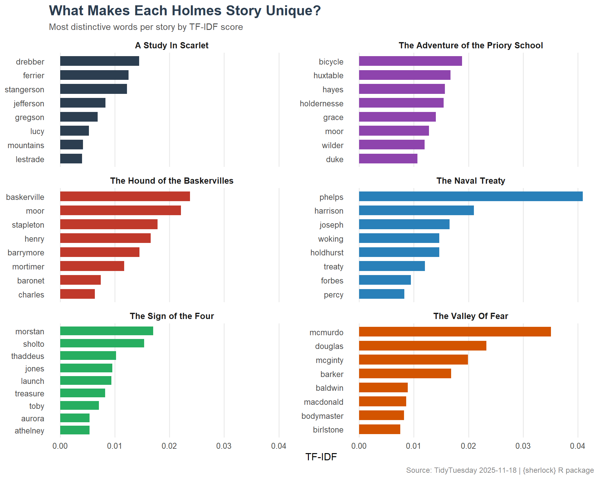
Which words are most unique to each story compared to the rest of the canon?
book_words <- holmes_words %>%count(book, word, sort =TRUE)book_tfidf <- book_words %>%bind_tf_idf(word, book, n) %>%arrange(desc(tf_idf))# Top 3 distinctive words per book (sample of books)top_books <- book_lengths %>%head(6) %>%pull(book)book_tfidf %>%filter(book %in% top_books) %>%group_by(book) %>%slice_max(tf_idf, n =5) %>%select(book, word, tf_idf)
# A tibble: 30 × 3
# Groups:   book [6]
   book                               word         tf_idf
   <chr>                              <chr>         <dbl>
 1 A Study In Scarlet                 drebber     0.0144
 2 A Study In Scarlet                 ferrier     0.0125
 3 A Study In Scarlet                 stangerson  0.0123
 4 A Study In Scarlet                 jefferson   0.00828
 5 A Study In Scarlet                 gregson     0.00684
 6 The Adventure of the Priory School bicycle     0.0188
 7 The Adventure of the Priory School huxtable    0.0167
 8 The Adventure of the Priory School hayes       0.0157
 9 The Adventure of the Priory School holdernesse 0.0155
10 The Adventure of the Priory School grace       0.0140
# ℹ 20 more rows
Visualizing the Sentiment Arc of a Holmes Mystery
# Victorian-inspired paletteggplot(avg_arc, aes(x = decile, y = mean_sentiment)) +geom_area(fill ="#2C3E50", alpha =0.3) +geom_line(color ="#2C3E50", linewidth =1.2) +geom_point(color ="#C0392B", size =3) +geom_hline(yintercept =0, linetype ="dashed", color ="#777777") +annotate("text", x =0.05, y =max(avg_arc$mean_sentiment) *0.9,label ="More positive", hjust =0, size =3.5, color ="#27AE60", fontface ="italic" ) +annotate("text", x =0.05, y =min(avg_arc$mean_sentiment) *0.9,label ="More negative", hjust =0, size =3.5, color ="#C0392B", fontface ="italic" ) +scale_x_continuous(labels = scales::percent_format(),breaks =seq(0, 1, 0.1) ) +labs(title ="The Emotional Arc of a Sherlock Holmes Mystery",subtitle ="Average net sentiment (Bing lexicon) across story progression | All stories combined",x ="Story Progress",y ="Net Sentiment",caption ="Source: TidyTuesday 2025-11-18 | {sherlock} R package by Emil Hvitfeldt" ) +theme_minimal(base_size =13) +theme(plot.title =element_text(face ="bold", size =18, color ="#2C3E50"),plot.subtitle =element_text(size =11, color ="#555555"),plot.caption =element_text(size =9, color ="#888888"),panel.grid.minor =element_blank() )
tfidf_plot <- book_tfidf %>%filter(book %in% top_books) %>%group_by(book) %>%slice_max(tf_idf, n =8) %>%ungroup() %>%mutate(word =reorder_within(word, tf_idf, book) )ggplot(tfidf_plot, aes(x = word, y = tf_idf, fill = book)) +geom_col(show.legend =FALSE, width =0.7) +facet_wrap(~ book, scales ="free_y", ncol =2) +scale_x_reordered() +scale_fill_manual(values =c("#2C3E50", "#8E44AD", "#C0392B", "#2980B9", "#27AE60", "#D35400" )) +coord_flip() +labs(title ="What Makes Each Holmes Story Unique?",subtitle ="Most distinctive words per story by TF-IDF score",x =NULL,y ="TF-IDF",caption ="Source: TidyTuesday 2025-11-18 | {sherlock} R package" ) +theme_minimal(base_size =12) +theme(plot.title =element_text(face ="bold", size =17, color ="#2C3E50"),plot.subtitle =element_text(size =11, color ="#555555"),plot.caption =element_text(size =9, color ="#888888"),strip.text =element_text(face ="bold", size =10),panel.grid.major.y =element_blank(),panel.grid.minor =element_blank() )
Final thoughts and takeaways
The complete Sherlock Holmes canon — 56 short stories and 4 novels — reveals remarkably consistent patterns when viewed through a computational lens. The average sentiment arc across all stories follows a recognizable shape: stories tend to open with moderate positivity (Watson setting the scene), dip into negativity during the middle act (the mystery deepens, danger emerges), and recover toward resolution.
The TF-IDF analysis surfaces the unique vocabulary fingerprint of each story. Names, locations, and domain-specific terms (poisons, weapons, occupations) define each mystery’s identity. This is Conan Doyle’s formula: each story inhabits a distinct world even while following the same narrative structure.
Note
The Bing sentiment lexicon is a blunt instrument for Victorian prose. Words like “grave” and “dark” carry different connotations in 1890s London than in modern usage. A more nuanced analysis might use a period-appropriate lexicon or train a custom sentiment model on 19th-century fiction.