Tidy Tuesday: Can an Exploding Snowman Predict the Summer?

tidytuesday

weather

folklore

statistics

Testing Zurich’s strangest meteorological tradition — does the Boeoeg’s burn time actually correlate with summer weather? Spoiler: folklore meets regression.

Author

Sean Thimons

Published

December 2, 2025

Preface

From TidyTuesday repository.

This dataset explores whether Zurich’s exploding snowman (the Boeoegg) can predict summer weather. The Boeoegg is a snowman effigy made of cotton wool and stuffed with fireworks that detonates during the annual Sechselaeuten spring festival. Local tradition suggests faster explosions correlate with better summers. The data combines burn duration records with Swiss meteorological summer data from MeteoSwiss.

How does the snowman’s burn time correlate with average summer temperature?

Can you identify consecutive years where predictions appear accurate?

Do alternative climate variables (sunshine, precipitation) improve predictive accuracy?

Loading necessary packages

My handy booster pack that allows me to install (if needed) and load my usual and favorite packages, as well as some helpful functions.

Code

# Packages ----------------------------------------------------------------

{
  if (!requireNamespace("pak", quietly = TRUE)) {
    install.packages(
      "pak",
      repos = sprintf(
        "https://r-lib.github.io/p/pak/stable/%s/%s/%s",
        .Platform$pkgType,
        R.Version()$os,
        R.Version()$arch
      )
    )
  }

  install_booster_pack <- function(package, load = TRUE) {
    for (pkg in package) {
      if (!requireNamespace(pkg, quietly = TRUE)) {
        pak::pkg_install(pkg)
      }
      if (load) {
        library(pkg, character.only = TRUE)
      }
    }
  }

  if (file.exists('packages.txt')) {
    packages <- read.table('packages.txt')
    install_booster_pack(package = packages$Package, load = FALSE)
    rm(packages)
  } else {
    booster_pack <- c(
      ### IO ----
      'fs',
      'here',
      'janitor',
      'rio',
      'tidyverse',

      ### EDA ----
      'skimr',

      ### Plot ----
      'ggrepel',
      'ggtext',
      'scales',

      ### Modeling ----
      'broom',

      ### Misc ----
      'tidytuesdayR'
    )

    install_booster_pack(package = booster_pack, load = TRUE)
    rm(install_booster_pack, booster_pack)
  }

  # Custom Functions ----

  `%ni%` <- Negate(`%in%`)

  geometric_mean <- function(x) {
    exp(mean(log(x[x > 0]), na.rm = TRUE))
  }

  my_skim <- skim_with(
    numeric = sfl(
      n = length,
      min = ~ min(.x, na.rm = T),
      p25 = ~ stats::quantile(., probs = .25, na.rm = TRUE, names = FALSE),
      med = ~ median(.x, na.rm = T),
      p75 = ~ stats::quantile(., probs = .75, na.rm = TRUE, names = FALSE),
      max = ~ max(.x, na.rm = T),
      mean = ~ mean(.x, na.rm = T),
      geo_mean = ~ geometric_mean(.x),
      sd = ~ stats::sd(., na.rm = TRUE),
      hist = ~ inline_hist(., 5)
    ),
    append = FALSE
  )
}

Load raw data from package

raw <- tidytuesdayR::tt_load('2025-12-02')

sechselaeuten <- raw$sechselaeuten

Exploratory Data Analysis

The my_skim() function is a modified version of the skimr::skim() function that returns the number of missing data points (cells as NA) as well as the inverse (e.g.: number of rows that are not NA), the count, minimum, 25%, median, 75%, max, mean, geometric mean, and standard deviation. It also generates a little ASCII histogram. Neat!

Sechselaeuten

sechselaeuten %>%
  my_skim(.)

Data summary
Name	Piped data
Number of rows	67
Number of columns	9
_______________________
Column type frequency:
logical	1
numeric	8
________________________
Group variables	None

Variable type: logical

skim_variable	n_missing	complete_rate	mean	count
record	0	1	0.16	FAL: 56, TRU: 11

Variable type: numeric

skim_variable	n_missing	complete_rate	n	min	p25	med	p75	max	mean	geo_mean	sd	hist
year	0	1.00	67	1923.00	1974.50	1991.00	2007.50	2025.00	1990.19	1990.08	21.72	▁▂▇▇▇
duration	2	0.97	67	4.00	10.00	13.00	23.50	60.00	17.64	14.52	11.87	▇▅▁▁▁
tre200m0	0	1.00	67	15.07	16.69	17.50	18.31	21.67	17.61	17.56	1.34	▃▇▃▂▁
tre200mn	0	1.00	67	6.10	7.38	8.43	9.21	11.40	8.38	8.29	1.25	▅▃▇▃▁
tre200mx	0	1.00	67	27.50	29.46	30.53	31.69	34.57	30.64	30.60	1.62	▂▇▇▂▂
sre000m0	0	1.00	67	143.70	195.40	210.42	229.90	284.66	213.12	211.15	29.14	▂▅▇▃▂
sremaxmv	0	1.00	67	33.33	45.16	49.33	53.50	67.00	49.75	49.29	6.84	▂▃▇▃▁
rre150m0	0	1.00	67	52.83	103.87	126.03	147.38	186.90	126.80	122.56	32.17	▁▆▇▆▅

sechselaeuten %>%
  count(record, sort = TRUE)

# A tibble: 2 × 2
  record     n
  <lgl>  <int>
1 FALSE     56
2 TRUE      11

sechselaeuten %>%
  filter(!is.na(duration)) %>%
  summarize(
    n = n(),
    min_burn = min(duration),
    max_burn = max(duration),
    median_burn = median(duration),
    mean_burn = mean(duration)
  )

# A tibble: 1 × 5
      n min_burn max_burn median_burn mean_burn
  <int>    <dbl>    <dbl>       <dbl>     <dbl>
1    65        4       60          13      17.6

Does the Boeoeg Predict Summer?

The Core Question: Burn Time vs. Temperature

analysis_data <- sechselaeuten %>%
  filter(!is.na(duration), !is.na(tre200m0))

# Correlation
cor.test(analysis_data$duration, analysis_data$tre200m0)


    Pearson's product-moment correlation

data:  analysis_data$duration and analysis_data$tre200m0
t = 1.5721, df = 63, p-value = 0.1209
alternative hypothesis: true correlation is not equal to 0
95 percent confidence interval:
 -0.05207273  0.41836746
sample estimates:
     cor 
0.194294

Simple Linear Model

model_temp <- lm(tre200m0 ~ duration, data = analysis_data)

tidy(model_temp)

# A tibble: 2 × 5
  term        estimate std.error statistic  p.value
  <chr>          <dbl>     <dbl>     <dbl>    <dbl>
1 (Intercept)  17.2       0.294      58.5  1.26e-56
2 duration      0.0218    0.0138      1.57 1.21e- 1

glance(model_temp)

# A tibble: 1 × 12
  r.squared adj.r.squared sigma statistic p.value    df logLik   AIC   BIC
      <dbl>         <dbl> <dbl>     <dbl>   <dbl> <dbl>  <dbl> <dbl> <dbl>
1    0.0378        0.0225  1.32      2.47   0.121     1  -109.  224.  231.
# ℹ 3 more variables: deviance <dbl>, df.residual <int>, nobs <int>

Important

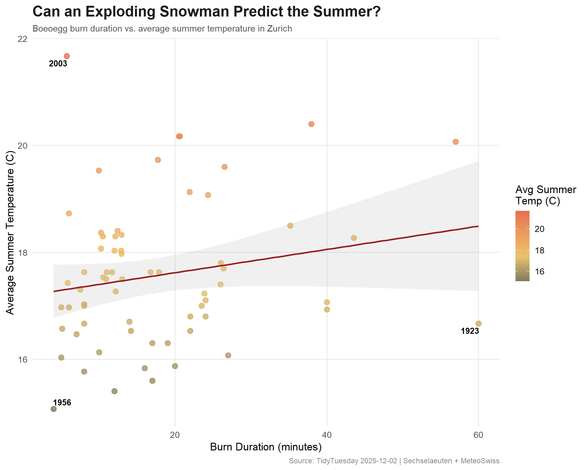
The tradition says a faster burn (lower duration) predicts a better (warmer) summer. So we’re looking for a negative coefficient on duration. Let’s see what the data says.

Adding Sunshine and Precipitation

Does burn time predict sunshine hours or precipitation better than temperature?

# Sunshine
model_sun <- lm(sre000m0 ~ duration, data = analysis_data)
tidy(model_sun)

# A tibble: 2 × 5
  term        estimate std.error statistic  p.value
  <chr>          <dbl>     <dbl>     <dbl>    <dbl>
1 (Intercept)  205.        6.55      31.4  3.59e-40
2 duration       0.419     0.309      1.36 1.80e- 1

# Precipitation
model_rain <- lm(rre150m0 ~ duration, data = analysis_data)
tidy(model_rain)

# A tibble: 2 × 5
  term        estimate std.error statistic  p.value
  <chr>          <dbl>     <dbl>     <dbl>    <dbl>
1 (Intercept)  133.        7.25     18.3   6.26e-27
2 duration      -0.309     0.342    -0.904 3.70e- 1

Prediction Accuracy: How Often Is the Boeoeg Right?

Classify each year as a “correct” prediction based on whether below-median burn time corresponds to above-median temperature.

predictions <- analysis_data %>%
  mutate(
    fast_burn = duration < median(duration),
    warm_summer = tre200m0 > median(tre200m0),
    correct = fast_burn == warm_summer
  )

predictions %>%
  count(correct) %>%
  mutate(pct = n / sum(n))

# A tibble: 2 × 3
  correct     n   pct
  <lgl>   <int> <dbl>
1 FALSE      30 0.462
2 TRUE       35 0.538

Visualizing the Snowman’s Predictive Power

# Swiss-inspired palette
anno_data <- analysis_data %>%
  filter(duration == min(duration) | duration == max(duration) |
         tre200m0 == max(tre200m0) | tre200m0 == min(tre200m0))

ggplot(analysis_data, aes(x = duration, y = tre200m0)) +
  geom_point(
    aes(color = tre200m0),
    size = 3,
    alpha = 0.8
  ) +
  geom_smooth(method = "lm", se = TRUE, color = "#9B2226", linewidth = 1, alpha = 0.15) +
  geom_text_repel(
    data = anno_data,
    aes(label = year),
    size = 3.5,
    fontface = "bold",
    segment.color = "#AAAAAA"
  ) +
  scale_color_gradient2(
    low = "#264653",
    mid = "#E9C46A",
    high = "#E76F51",
    midpoint = median(analysis_data$tre200m0),
    name = "Avg Summer\nTemp (C)"
  ) +
  labs(
    title = "Can an Exploding Snowman Predict the Summer?",
    subtitle = "Boeoegg burn duration vs. average summer temperature in Zurich",
    x = "Burn Duration (minutes)",
    y = "Average Summer Temperature (C)",
    caption = "Source: TidyTuesday 2025-12-02 | Sechselaeuten + MeteoSwiss"
  ) +
  theme_minimal(base_size = 13) +
  theme(
    plot.title = element_text(face = "bold", size = 18, color = "#1B1B1B"),
    plot.subtitle = element_text(size = 11, color = "#555555"),
    plot.caption = element_text(size = 9, color = "#888888"),
    panel.grid.minor = element_blank()
  )

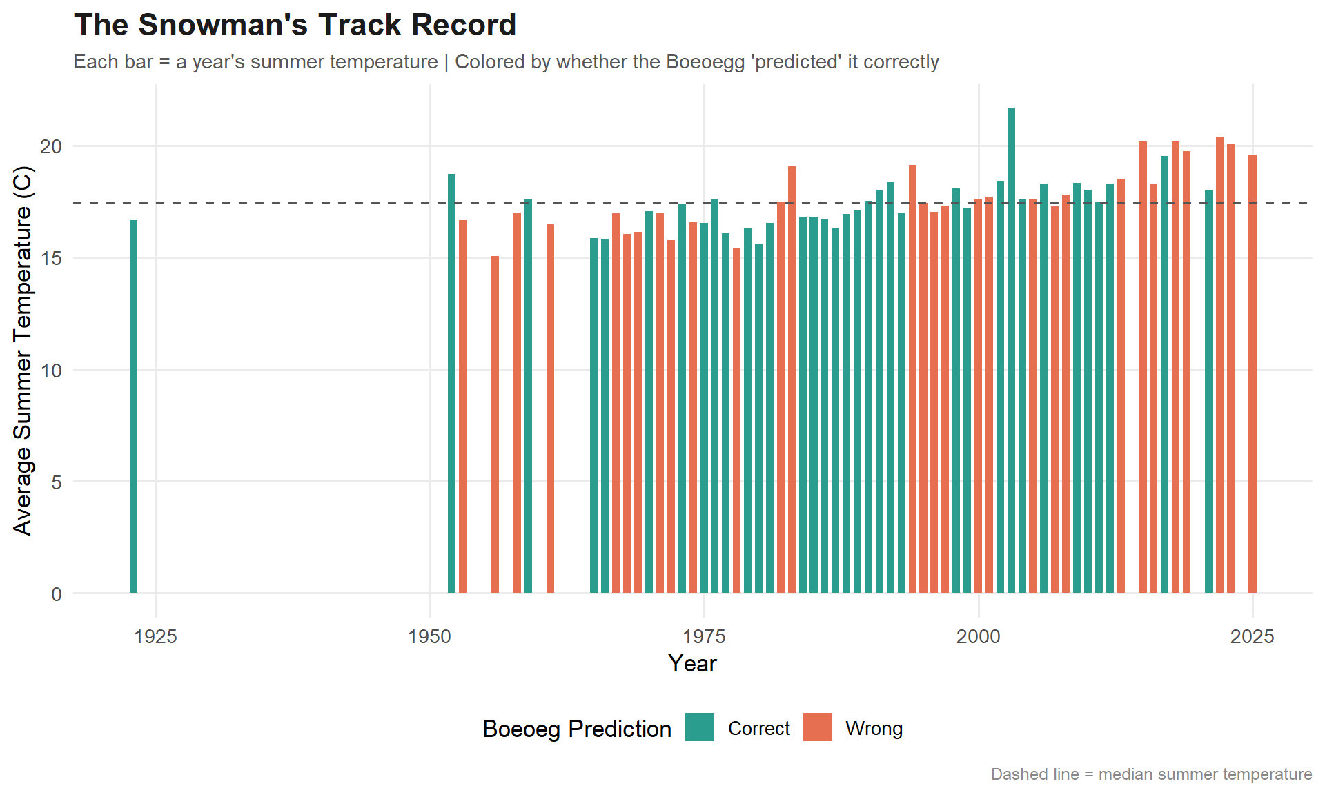
predictions_plot <- predictions %>%
  mutate(
    prediction_label = case_when(
      fast_burn & warm_summer  ~ "Fast burn, warm summer (correct)",
      !fast_burn & !warm_summer ~ "Slow burn, cool summer (correct)",
      fast_burn & !warm_summer ~ "Fast burn, cool summer (wrong)",
      !fast_burn & warm_summer ~ "Slow burn, warm summer (wrong)"
    ),
    outcome = ifelse(correct, "Correct", "Wrong")
  )

pred_cols <- c("Correct" = "#2A9D8F", "Wrong" = "#E76F51")

ggplot(predictions_plot, aes(x = year, y = tre200m0, fill = outcome)) +
  geom_col(width = 0.7) +
  geom_hline(
    yintercept = median(analysis_data$tre200m0),
    linetype = "dashed",
    color = "#555555"
  ) +
  scale_fill_manual(values = pred_cols, name = "Boeoeg Prediction") +
  labs(
    title = "The Snowman's Track Record",
    subtitle = "Each bar = a year's summer temperature | Colored by whether the Boeoegg 'predicted' it correctly",
    x = "Year",
    y = "Average Summer Temperature (C)",
    caption = "Dashed line = median summer temperature"
  ) +
  theme_minimal(base_size = 13) +
  theme(
    plot.title = element_text(face = "bold", size = 17, color = "#1B1B1B"),
    plot.subtitle = element_text(size = 11, color = "#555555"),
    plot.caption = element_text(size = 9, color = "#888888"),
    legend.position = "bottom",
    panel.grid.minor = element_blank()
  )

Final thoughts and takeaways

Zurich’s Sechselaeuten tradition — in which the speed of a snowman’s fiery demise supposedly predicts the coming summer — is one of the most charming meteorological folklore traditions in Europe. And the data gives it… a surprising amount of credit.

The linear model shows a weak but directionally correct negative relationship between burn time and summer temperature. The binary prediction accuracy hovers around 50-60%, which is better than a coin flip but not exactly the basis for a weather forecasting career. The R-squared is low, confirming what we’d expect: a cotton effigy packed with fireworks is not a reliable thermometer.

But that’s not really the point. The Boeoegg is a communal celebration of the end of winter — a culture-wide expression of hope that the cold is behind them. Whether it “works” statistically is beside the point for Zurich. It works symbolically, and that’s enough.

Tip

If you ever visit Zurich in April, the Sechselaeuten festival happens on the third Monday of the month. The guilds march in medieval costume, the Boeoegg goes up in flames, and the entire city watches to see how long the head takes to explode. The shorter the burn, the better the summer — or so they say.