A modern take on the classic car dataset — exploring price, performance, and powertrain trends for vehicles available in Qatar’s 2025 market, with metric measurements and global representation.
This dataset provides a modern, internationally-focused alternative to classic datasets like mtcars and mpg. Collected in early 2025 by Paul Musgrave and students from Georgetown University’s international politics program in Qatar, it contains pricing data for cars available in Qatar using SI units, featuring contemporary vehicle types including electric and hybrid models.
What patterns emerge in price distribution?
How do logged price and performance metrics correlate?
Do manufacturing origins show differences in pricing or electric vehicle prevalence?
What relationships exist between vehicle dimensions and seating/trunk capacity?
Loading necessary packages
My handy booster pack that allows me to install (if needed) and load my usual and favorite packages, as well as some helpful functions.
raw <- tidytuesdayR::tt_load('2025-12-09')cars <- raw$qatarcars
Exploratory Data Analysis
The my_skim() function is a modified version of the skimr::skim() function that returns the number of missing data points (cells as NA) as well as the inverse (e.g.: number of rows that are notNA), the count, minimum, 25%, median, 75%, max, mean, geometric mean, and standard deviation. It also generates a little ASCII histogram. Neat!
Cars
cars %>%my_skim(.)
Data summary
Name
Piped data
Number of rows
105
Number of columns
15
_______________________
Column type frequency:
character
5
numeric
10
________________________
Group variables
None
Variable type: character
skim_variable
n_missing
complete_rate
min
max
empty
n_unique
whitespace
origin
0
1
2
11
0
8
0
make
0
1
2
10
0
31
0
model
0
1
1
20
0
105
0
type
0
1
3
9
0
4
0
enginetype
0
1
6
8
0
3
0
Variable type: numeric
skim_variable
n_missing
complete_rate
n
min
p25
med
p75
max
mean
geo_mean
sd
hist
length
0
1.0
105
3.60
4.50
4.68
4.85
5.470e+00
4.66
4.65
0.35
▁▂▇▇▂
width
0
1.0
105
1.59
1.82
1.88
1.98
4.630e+00
1.91
1.90
0.30
▇▁▁▁▁
height
0
1.0
105
1.12
1.46
1.54
1.69
2.000e+00
1.57
1.56
0.19
▂▇▇▇▃
seating
0
1.0
105
2.00
5.00
5.00
5.00
8.000e+00
5.01
4.83
1.20
▁▁▇▁▂
trunk
0
1.0
105
0.00
284.00
448.00
542.00
1.233e+03
437.65
379.70
264.69
▅▇▆▂▁
economy
10
0.9
105
1.20
6.50
7.60
10.65
2.250e+01
8.70
8.06
3.58
▂▇▃▁▁
horsepower
0
1.0
105
76.00
154.00
248.00
380.00
1.973e+03
317.78
249.13
289.88
▇▂▁▁▁
price
0
1.0
105
35000.00
91000.00
164000.00
310000.00
3.300e+07
796573.15
190496.60
3530840.76
▇▁▁▁▁
mass
0
1.0
105
945.00
1428.00
1701.00
2055.00
2.746e+03
1776.41
1714.61
471.56
▅▇▇▅▃
performance
0
1.0
105
2.40
4.80
6.90
8.80
1.450e+01
7.10
6.53
2.84
▇▇▇▃▂
cars %>%count(origin, sort =TRUE)
# A tibble: 8 × 2
  origin          n
  <chr>       <int>
1 Japan          29
2 Germany        20
3 PR China       18
4 UK             11
5 South Korea    10
6 USA             9
7 Italy           5
8 Sweden          3
cars %>%count(make, sort =TRUE) %>%head(15)
# A tibble: 15 × 2
   make           n
   <chr>      <int>
 1 Toyota        10
 2 Kia            6
 3 BMW            5
 4 MG             5
 5 Mercedes       5
 6 Hyundai        4
 7 Lexus          4
 8 Mazda          4
 9 Mitsubishi     4
10 Volkswagen     4
11 Audi           3
12 Bentley        3
13 Cadillac       3
14 Chery          3
15 Ford           3
cars %>%count(type, sort =TRUE)
# A tibble: 4 × 2
  type          n
  <chr>     <int>
1 SUV          55
2 Sedan        28
3 Coupe        14
4 Hatchback     8
cars %>%count(enginetype, sort =TRUE)
# A tibble: 3 × 2
  enginetype     n
  <chr>      <int>
1 Petrol        81
2 Hybrid        14
3 Electric      10
A negative correlation between price and 0-100 km/h time means more expensive cars are faster (lower seconds = quicker acceleration). This is expected but the strength of the relationship varies by vehicle type.
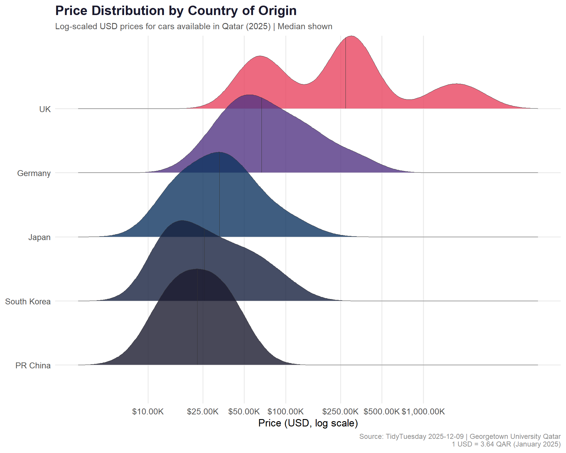
# Automotive-inspired palette: dark metals and accent colorstop_origins <- cars %>%count(origin, sort =TRUE) %>%filter(n >=10) %>%pull(origin)plot_data <- cars %>%filter(origin %in% top_origins, !is.na(price_usd)) %>%mutate(origin =fct_reorder(origin, price_usd, .fun = median))ggplot(plot_data, aes(x = price_usd, y = origin, fill = origin)) +geom_density_ridges(alpha =0.8,scale =1.5,quantile_lines =TRUE,quantiles =2,color ="#333333",linewidth =0.3 ) +scale_x_log10(labels = scales::dollar_format(prefix ="$", suffix ="K", scale =0.001),breaks =c(10000, 25000, 50000, 100000, 250000, 500000, 1000000) ) +scale_fill_manual(values =c("#1A1A2E", "#16213E", "#0F3460", "#533483","#E94560", "#B55400", "#2A9D8F", "#264653","#6A4C93", "#F4A261", "#344E41", "#E76F51" ) ) +labs(title ="Price Distribution by Country of Origin",subtitle ="Log-scaled USD prices for cars available in Qatar (2025) | Median shown",x ="Price (USD, log scale)",y =NULL,caption ="Source: TidyTuesday 2025-12-09 | Georgetown University Qatar\n1 USD = 3.64 QAR (January 2025)" ) +theme_minimal(base_size =13) +theme(plot.title =element_text(face ="bold", size =17, color ="#1A1A2E"),plot.subtitle =element_text(size =11, color ="#555555"),plot.caption =element_text(size =9, color ="#888888"),legend.position ="none",panel.grid.minor =element_blank() )
engine_cols <-c("petrol"="#E76F51","electric"="#2A9D8F","hybrid"="#E9C46A","diesel"="#264653")scatter_data <- cars %>%filter(!is.na(performance), !is.na(price_usd), !is.na(enginetype)) %>%filter(enginetype %in%names(engine_cols))# Label some notable outlierslabel_data <- scatter_data %>%filter(price_usd >200000| performance <3.5) %>%mutate(label =paste(make, model))ggplot(scatter_data, aes(x = price_usd, y = performance, color = enginetype)) +geom_point(alpha =0.6, size =2) +geom_text_repel(data = label_data,aes(label = label),size =3,max.overlaps =8,segment.color ="#AAAAAA" ) +scale_x_log10(labels = scales::dollar_format(prefix ="$", suffix ="K", scale =0.001)) +scale_y_reverse() +scale_color_manual(values = engine_cols, name ="Engine Type") +labs(title ="Money Buys Speed — But Powertrain Matters",subtitle ="0-100 km/h time vs. price by engine type | Lower = faster",x ="Price (USD, log scale)",y ="0–100 km/h (seconds)",caption ="Source: TidyTuesday 2025-12-09 | Georgetown University Qatar" ) +theme_minimal(base_size =13) +theme(plot.title =element_text(face ="bold", size =17, color ="#1A1A2E"),plot.subtitle =element_text(size =11, color ="#555555"),plot.caption =element_text(size =9, color ="#888888"),legend.position ="bottom",panel.grid.minor =element_blank() )
Final thoughts and takeaways
Qatar’s car market is a fascinating lens into global automotive trends. The dataset — designed as a modern, metric-first replacement for mtcars — reveals a market where luxury is the norm, not the exception. European manufacturers command the highest median prices, while Japanese and Korean brands dominate the volume segment with competitive pricing.
The performance-vs-price scatter reveals a clear but noisy relationship: money buys acceleration, but electric vehicles punch above their weight class. EVs cluster toward the faster end of their price range, reflecting the inherent torque advantage of electric motors. Qatar’s EV adoption story is still early, but the models available are competitive.
Tip
This dataset uses SI units throughout — liters per 100 km for economy, kilograms for mass, meters for dimensions. If you’re accustomed to mpg and pounds, the Qatari market data is a refreshing reminder that “car data” doesn’t have to mean “American car data.”