Tidy Tuesday: Roundabouts Across the World

tidytuesday
R
infrastructure
geography
Exploring the global spread of roundabouts — how has construction evolved over time, which countries lead adoption, and what types of intersections are being replaced?
Author

Sean Thimons

Published

December 16, 2025

Preface

From TidyTuesday repository.

This dataset comes from the {roundabouts} R package by Emil Hvitfeldt, which accesses the Kittelson & Associates roundabouts database. The database includes over 20,000 records documenting roundabout locations, configurations, and construction details worldwide.

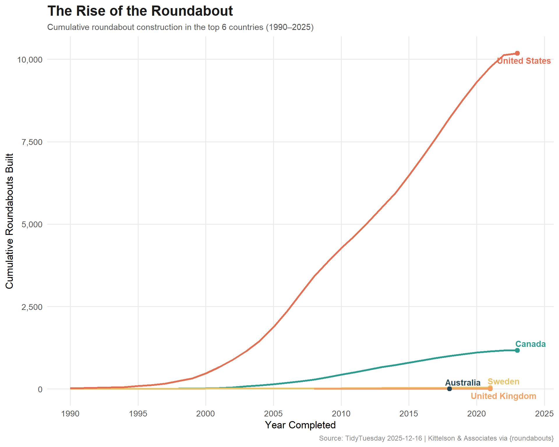
  • How has roundabout construction evolved over time, and are certain regions adopting them faster than others?
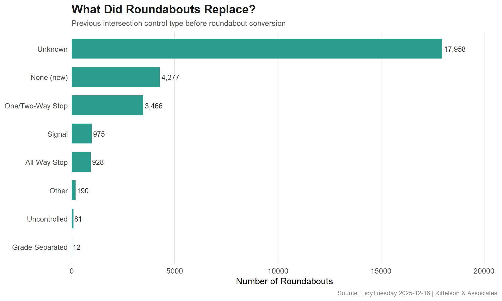
  • What intersection types are most commonly converted to roundabouts?
  • Which roundabouts feature the most unusual configurations?

Loading necessary packages

My handy booster pack that allows me to install (if needed) and load my usual and favorite packages, as well as some helpful functions.

Code
# Packages ----------------------------------------------------------------

{
  if (!requireNamespace("pak", quietly = TRUE)) {
    install.packages(
      "pak",
      repos = sprintf(
        "https://r-lib.github.io/p/pak/stable/%s/%s/%s",
        .Platform$pkgType,
        R.Version()$os,
        R.Version()$arch
      )
    )
  }

  install_booster_pack <- function(package, load = TRUE) {
    for (pkg in package) {
      if (!requireNamespace(pkg, quietly = TRUE)) {
        pak::pkg_install(pkg)
      }
      if (load) {
        library(pkg, character.only = TRUE)
      }
    }
  }

  if (file.exists('packages.txt')) {
    packages <- read.table('packages.txt')
    install_booster_pack(package = packages$Package, load = FALSE)
    rm(packages)
  } else {
    booster_pack <- c(
      ### IO ----
      'fs',
      'here',
      'janitor',
      'rio',
      'tidyverse',

      ### EDA ----
      'skimr',

      ### Plot ----
      'ggrepel',
      'ggtext',
      'scales',

      ### Misc ----
      'tidytuesdayR'
    )

    install_booster_pack(package = booster_pack, load = TRUE)
    rm(install_booster_pack, booster_pack)
  }

  # Custom Functions ----

  `%ni%` <- Negate(`%in%`)

  geometric_mean <- function(x) {
    exp(mean(log(x[x > 0]), na.rm = TRUE))
  }

  my_skim <- skim_with(
    numeric = sfl(
      n = length,
      min = ~ min(.x, na.rm = T),
      p25 = ~ stats::quantile(., probs = .25, na.rm = TRUE, names = FALSE),
      med = ~ median(.x, na.rm = T),
      p75 = ~ stats::quantile(., probs = .75, na.rm = TRUE, names = FALSE),
      max = ~ max(.x, na.rm = T),
      mean = ~ mean(.x, na.rm = T),
      geo_mean = ~ geometric_mean(.x),
      sd = ~ stats::sd(., na.rm = TRUE),
      hist = ~ inline_hist(., 5)
    ),
    append = FALSE
  )
}

Load raw data from package

raw <- tidytuesdayR::tt_load('2025-12-16')

roundabouts <- raw$roundabouts_clean

Exploratory Data Analysis

The my_skim() function is a modified version of the skimr::skim() function that returns the number of missing data points (cells as NA) as well as the inverse (e.g.: number of rows that are not NA), the count, minimum, 25%, median, 75%, max, mean, geometric mean, and standard deviation. It also generates a little ASCII histogram. Neat!

Roundabouts

roundabouts %>%
  my_skim(.)
Data summary
Name Piped data
Number of rows 27887
Number of columns 18
_______________________
Column type frequency:
character 13
numeric 5
________________________
Group variables None

Variable type: character

skim_variable n_missing complete_rate min max empty n_unique whitespace
name 0 1.00 4 154 0 27612 0
address 0 1.00 12 99 0 9166 0
town_city 2 1.00 2 46 0 7845 0
county_area 91 1.00 3 57 0 2954 0
state_region 1415 0.95 3 41 0 580 0
country 0 1.00 4 24 0 119 0
type 0 1.00 5 28 0 6 0
status 0 1.00 7 8 0 3 0
lane_type 0 1.00 7 50 0 9 0
functional_class 0 1.00 7 31 0 3 0
control_type 0 1.00 5 20 0 7 0
other_control_type 0 1.00 4 75 0 12 0
previous_control_type 0 1.00 5 16 0 8 0

Variable type: numeric

skim_variable n_missing complete_rate n min p25 med p75 max mean geo_mean sd hist
lat 0 1 27887 -170.72 -88.09 -71.46 17.92 178.47 -18.88 37.49 90.85 ▃▇▆▁▃
long 0 1 27887 -53.13 30.41 39.97 48.49 70.98 29.99 42.02 30.46 ▂▁▁▇▅
year_completed 0 1 27887 0.00 0.00 0.00 2010.00 2023.00 830.91 2011.41 990.44 ▇▁▁▁▆
approaches 0 1 27887 0.00 3.00 4.00 4.00 12.00 3.68 3.65 0.67 ▁▇▁▁▁
driveways 0 1 27887 0.00 0.00 0.00 0.00 19.00 0.07 1.30 0.48 ▇▁▁▁▁
roundabouts %>%
  count(country, sort = TRUE) %>%
  head(15)
# A tibble: 15 × 2
   country            n
   <chr>          <int>
 1 United States  12952
 2 Australia       3720
 3 United Kingdom  1777
 4 Sweden          1553
 5 Canada          1246
 6 New Zealand      861
 7 Netherlands      760
 8 Russia           472
 9 Norway           467
10 France           384
11 Spain            374
12 Italy            241
13 Poland           218
14 Ireland          211
15 Finland          194
roundabouts %>%
  count(type, sort = TRUE)
# A tibble: 6 × 2
  type                             n
  <chr>                        <int>
1 Roundabout                   23141
2 Other                         2928
3 Traffic Calming Circle         799
4 Unknown                        390
5 Signalized Roundabout/Circle   316
6 Rotary                         313
roundabouts %>%
  count(status, sort = TRUE)
# A tibble: 3 × 2
  status       n
  <chr>    <int>
1 Existing 27759
2 Unknown     72
3 Removed     56
roundabouts %>%
  count(previous_control_type, sort = TRUE) %>%
  head(10)
# A tibble: 8 × 2
  previous_control_type     n
  <chr>                 <int>
1 Unknown               17958
2 None (new)             4277
3 One/Two-Way Stop       3466
4 Signal                  975
5 All-Way Stop            928
6 Other                   190
7 Uncontrolled             81
8 Grade Separated          12

Roundabout Adoption Over Time

Construction Timeline

How has roundabout construction evolved over the decades?

yearly_builds <- roundabouts %>%
  filter(!is.na(year_completed), year_completed >= 1950, year_completed <= 2025) %>%
  count(year_completed, name = "n_built")

yearly_builds %>%
  arrange(desc(n_built)) %>%
  head(10)
# A tibble: 10 × 2
   year_completed n_built
            <dbl>   <int>
 1           2018     669
 2           2017     656
 3           2016     637
 4           2019     608
 5           2015     599
 6           2020     589
 7           2008     583
 8           2007     575
 9           2006     530
10           2013     515

Top Countries Over Time

Which countries have been building the most roundabouts, and how does their adoption curve differ?

top_countries <- roundabouts %>%
  count(country, sort = TRUE) %>%
  head(6) %>%
  pull(country)

country_timeline <- roundabouts %>%
  filter(
    country %in% top_countries,
    !is.na(year_completed),
    year_completed >= 1990,
    year_completed <= 2025
  ) %>%
  count(country, year_completed, name = "n_built") %>%
  group_by(country) %>%
  mutate(cumulative = cumsum(n_built)) %>%
  ungroup()

country_timeline %>%
  group_by(country) %>%
  slice_max(year_completed, n = 1) %>%
  arrange(desc(cumulative))
# A tibble: 5 × 4
# Groups:   country [5]
  country        year_completed n_built cumulative
  <chr>                   <dbl>   <int>      <int>
1 United States            2023      54      10181
2 Canada                   2023       2       1171
3 Sweden                   2021       2         38
4 United Kingdom           2021       1          3
5 Australia                2018       1          2

What Gets Replaced?

What types of intersections are most commonly converted to roundabouts?

conversions <- roundabouts %>%
  filter(!is.na(previous_control_type), previous_control_type != "unknown") %>%
  count(previous_control_type, sort = TRUE) %>%
  mutate(pct = n / sum(n))

conversions
# A tibble: 8 × 3
  previous_control_type     n      pct
  <chr>                 <int>    <dbl>
1 Unknown               17958 0.644   
2 None (new)             4277 0.153   
3 One/Two-Way Stop       3466 0.124   
4 Signal                  975 0.0350  
5 All-Way Stop            928 0.0333  
6 Other                   190 0.00681 
7 Uncontrolled             81 0.00290 
8 Grade Separated          12 0.000430

Visualizing the Rise of the Roundabout

# Infrastructure-inspired palette
country_cols <- c(
  "#264653",  # deep teal
  "#2A9D8F",  # muted teal
  "#E9C46A",  # warm yellow
  "#F4A261",  # sandy orange
  "#E76F51",  # burnt sienna
  "#6A4C93"   # muted purple
)

ggplot(country_timeline, aes(x = year_completed, y = cumulative, color = country)) +
  geom_line(linewidth = 1.2) +
  geom_point(
    data = country_timeline %>%
      group_by(country) %>%
      slice_max(year_completed, n = 1),
    size = 2.5
  ) +
  geom_text_repel(
    data = country_timeline %>%
      group_by(country) %>%
      slice_max(year_completed, n = 1),
    aes(label = country),
    nudge_x = 1,
    size = 3.8,
    fontface = "bold",
    direction = "y",
    segment.color = "#AAAAAA"
  ) +
  scale_x_continuous(breaks = seq(1990, 2025, 5)) +
  scale_y_continuous(labels = scales::comma) +
  scale_color_manual(values = country_cols) +
  labs(
    title = "The Rise of the Roundabout",
    subtitle = "Cumulative roundabout construction in the top 6 countries (1990–2025)",
    x = "Year Completed",
    y = "Cumulative Roundabouts Built",
    caption = "Source: TidyTuesday 2025-12-16 | Kittelson & Associates via {roundabouts}"
  ) +
  theme_minimal(base_size = 13) +
  theme(
    plot.title = element_text(face = "bold", size = 18, color = "#1B1B1B"),
    plot.subtitle = element_text(size = 11, color = "#555555"),
    plot.caption = element_text(size = 9, color = "#888888"),
    legend.position = "none",
    panel.grid.minor = element_blank()
  )

conversions_plot <- conversions %>%
  filter(n >= 10) %>%
  mutate(previous_control_type = fct_reorder(previous_control_type, n))

ggplot(conversions_plot, aes(x = previous_control_type, y = n)) +
  geom_col(fill = "#2A9D8F", width = 0.7) +
  geom_text(aes(label = scales::comma(n)), hjust = -0.1, size = 3.5, color = "#333333") +
  scale_y_continuous(expand = expansion(mult = c(0, 0.15))) +
  coord_flip() +
  labs(
    title = "What Did Roundabouts Replace?",
    subtitle = "Previous intersection control type before roundabout conversion",
    x = NULL,
    y = "Number of Roundabouts",
    caption = "Source: TidyTuesday 2025-12-16 | Kittelson & Associates"
  ) +
  theme_minimal(base_size = 13) +
  theme(
    plot.title = element_text(face = "bold", size = 17, color = "#1B1B1B"),
    plot.subtitle = element_text(size = 11, color = "#555555"),
    plot.caption = element_text(size = 9, color = "#888888"),
    panel.grid.major.y = element_blank(),
    panel.grid.minor = element_blank()
  )

Final thoughts and takeaways

The global adoption of roundabouts tells a fascinating story of traffic engineering evolution. The United States — long a holdout in the roundabout revolution — has undergone a dramatic shift, with construction accelerating sharply from the mid-2000s onward. This tracks with mounting safety research showing roundabouts reduce fatal and injury crashes by 78-82% compared to traditional signalized intersections.

The “what did they replace?” analysis reveals that stop signs and traffic signals are the most common predecessors, suggesting that planners are targeting existing problem intersections rather than building roundabouts into greenfield developments. This is a retrofit story — cities learning from crash data and choosing a safer geometry.

Note

The Kittelson database, while extensive, has known biases in its coverage. English-speaking countries are overrepresented relative to continental Europe, where roundabouts have been commonplace for decades. France alone has an estimated 30,000+ roundabouts — far more than appear in this database.