Tidy Tuesday: The Languages of the World

tidytuesday

linguistics

geography

endangerment

Exploring the world’s 8,000+ languages through Glottolog — which regions face the greatest endangerment, how do language families span the globe, and what patterns emerge from mapping linguistic diversity?

Author

Sean Thimons

Published

December 23, 2025

Preface

From TidyTuesday repository.

This week’s dataset comes from Glottolog 5.2.1, an open-access linguistics database maintained by the Max Planck Institute for Evolutionary Anthropology. The database encompasses over 8,000 languages of the world with details on names, genealogy, geography, and endangerment status.

Which macroareas have the highest concentration of endangered languages?

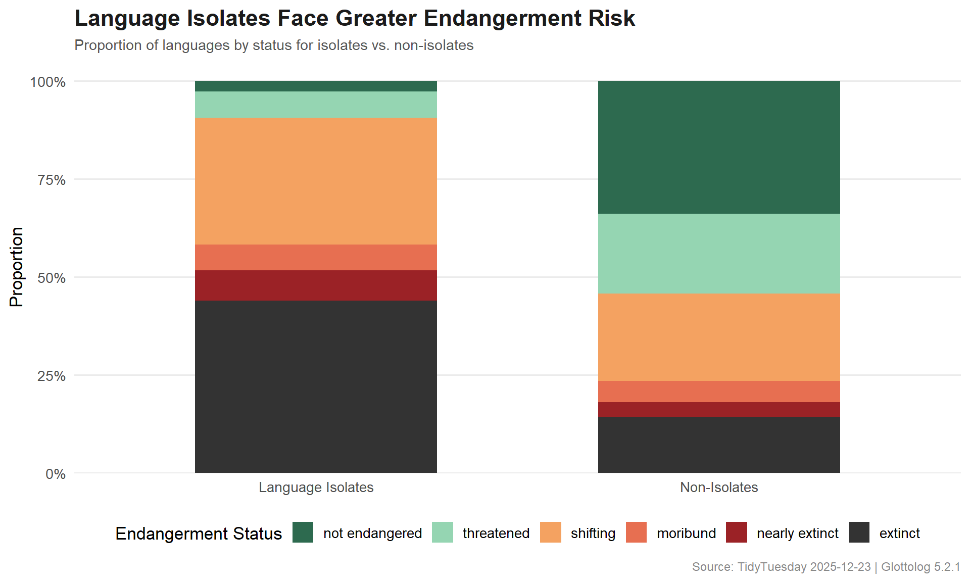
Are language isolates more likely to be endangered?

Which language families span the widest geographic range?

What geographic patterns emerge when mapping endangered languages?

Loading necessary packages

My handy booster pack that allows me to install (if needed) and load my usual and favorite packages, as well as some helpful functions.

Code

# Packages ----------------------------------------------------------------

{
  if (!requireNamespace("pak", quietly = TRUE)) {
    install.packages(
      "pak",
      repos = sprintf(
        "https://r-lib.github.io/p/pak/stable/%s/%s/%s",
        .Platform$pkgType,
        R.Version()$os,
        R.Version()$arch
      )
    )
  }

  install_booster_pack <- function(package, load = TRUE) {
    for (pkg in package) {
      if (!requireNamespace(pkg, quietly = TRUE)) {
        pak::pkg_install(pkg)
      }
      if (load) {
        library(pkg, character.only = TRUE)
      }
    }
  }

  if (file.exists('packages.txt')) {
    packages <- read.table('packages.txt')
    install_booster_pack(package = packages$Package, load = FALSE)
    rm(packages)
  } else {
    booster_pack <- c(
      ### IO ----
      'fs',
      'here',
      'janitor',
      'rio',
      'tidyverse',

      ### EDA ----
      'skimr',

      ### Plot ----
      'ggrepel',
      'ggtext',
      'scales',
      'patchwork',

      ### Misc ----
      'tidytuesdayR'
    )

    install_booster_pack(package = booster_pack, load = TRUE)
    rm(install_booster_pack, booster_pack)
  }

  # Custom Functions ----

  `%ni%` <- Negate(`%in%`)

  geometric_mean <- function(x) {
    exp(mean(log(x[x > 0]), na.rm = TRUE))
  }

  my_skim <- skim_with(
    numeric = sfl(
      n = length,
      min = ~ min(.x, na.rm = T),
      p25 = ~ stats::quantile(., probs = .25, na.rm = TRUE, names = FALSE),
      med = ~ median(.x, na.rm = T),
      p75 = ~ stats::quantile(., probs = .75, na.rm = TRUE, names = FALSE),
      max = ~ max(.x, na.rm = T),
      mean = ~ mean(.x, na.rm = T),
      geo_mean = ~ geometric_mean(.x),
      sd = ~ stats::sd(., na.rm = TRUE),
      hist = ~ inline_hist(., 5)
    ),
    append = FALSE
  )
}

Load raw data from package

raw <- tidytuesdayR::tt_load('2025-12-23')

languages <- raw$languages
families <- raw$families
endangered_status <- raw$endangered_status

Exploratory Data Analysis

The my_skim() function is a modified version of the skimr::skim() function that returns the number of missing data points (cells as NA) as well as the inverse (e.g.: number of rows that are not NA), the count, minimum, 25%, median, 75%, max, mean, geometric mean, and standard deviation. It also generates a little ASCII histogram. Neat!

Languages

languages %>%
  my_skim(.)

Data summary
Name	Piped data
Number of rows	8612
Number of columns	9
_______________________
Column type frequency:
character	6
logical	1
numeric	2
________________________
Group variables	None

Variable type: character

skim_variable	n_missing	complete_rate	min	max	n_unique
id	0	1.00	8	8	8612
name	0	1.00	1	58	8612
macroarea	224	0.97	6	28	10
iso639p3code	755	0.91	3	3	7857
countries	102	0.99	2	101	707
family_id	182	0.98	8	8	247

Variable type: logical

skim_variable	n_missing	complete_rate	mean	count
is_isolate	0	1	0.02	FAL: 8430, TRU: 182

Variable type: numeric

skim_variable	n_missing	complete_rate	n	min	p25	med	p75	max	mean	geo_mean	sd	hist
latitude	312	0.96	8612	-55.27	-5.02	6.54	20.19	73.14	8.55	13.40	19.15	▁▅▇▃▁
longitude	312	0.96	8612	-178.78	6.82	45.02	123.49	179.31	50.11	55.66	81.15	▁▃▇▅▇

languages %>%
  count(macroarea, sort = TRUE)

# A tibble: 11 × 2
   macroarea                        n
   <chr>                        <int>
 1 Africa                        2363
 2 Papunesia                     2177
 3 Eurasia                       2017
 4 North America                  767
 5 South America                  676
 6 Australia                      381
 7 <NA>                           224
 8 Africa;Eurasia                   4
 9 Africa;Eurasia;South America     1
10 Africa;North America             1
11 Eurasia;Papunesia                1

languages %>%
  count(is_isolate, sort = TRUE)

# A tibble: 2 × 2
  is_isolate     n
  <lgl>      <int>
1 FALSE       8430
2 TRUE         182

Endangerment Status

endangered_status %>%
  my_skim(.)

Data summary
Name	Piped data
Number of rows	8567
Number of columns	3
_______________________
Column type frequency:
character	2
numeric	1
________________________
Group variables	None

Variable type: character

skim_variable	n_missing	complete_rate	min	max	empty	n_unique	whitespace
id	0	1	8	8	0	8567	0
status_label	0	1	7	14	0	6	0

Variable type: numeric

skim_variable	n_missing	complete_rate	n	min	p25	med	p75	max	mean	geo_mean	sd	hist
status_code	0	1	8567	1	1	2	4	6	2.76	2.24	1.75	▇▃▁▁▂

endangered_status %>%
  count(status_label, sort = TRUE)

# A tibble: 6 × 2
  status_label       n
  <chr>          <int>
1 not endangered  2791
2 shifting        1933
3 threatened      1688
4 extinct         1341
5 moribund         461
6 nearly extinct   353

Language Families

families %>%
  my_skim(.)

Data summary
Name	Piped data
Number of rows	4832
Number of columns	2
_______________________
Column type frequency:
character	2
________________________
Group variables	None

Variable type: character

skim_variable	n_missing	complete_rate	min	max	empty	n_unique	whitespace
id	0	1	8	8	0	4832	0
family	0	1	2	52	0	4832	0

nrow(families)

[1] 4832

Endangerment Analysis

Joining Languages with Endangerment Status

lang_status <- languages %>%
  left_join(endangered_status, by = "id") %>%
  mutate(
    status_label = factor(
      status_label,
      levels = c(
        "not endangered",
        "threatened",
        "shifting",
        "moribund",
        "nearly extinct",
        "extinct"
      )
    )
  )

lang_status %>%
  count(status_label, sort = TRUE)

# A tibble: 7 × 2
  status_label       n
  <fct>          <int>
1 not endangered  2704
2 shifting        1835
3 threatened      1629
4 extinct         1225
5 <NA>             474
6 moribund         434
7 nearly extinct   311

Important

Not every language has an endangerment classification in this dataset. Languages with NA status are typically those without enough documentation to assess their vitality — which is itself a concerning signal.

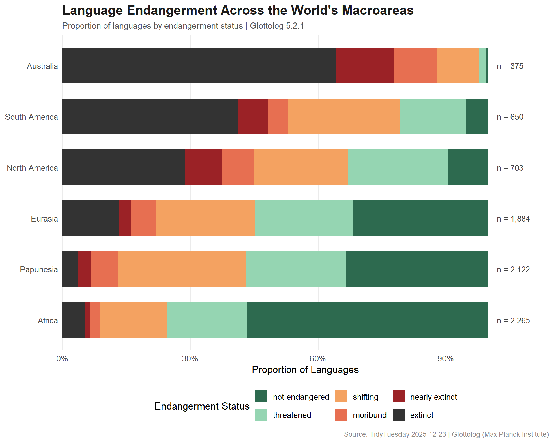
Endangerment by Macroarea

Which regions of the world face the greatest concentration of endangered languages?

region_danger <- lang_status %>%
  filter(!is.na(status_label), !is.na(macroarea), !grepl(";", macroarea)) %>%
  group_by(macroarea, status_label) %>%
  summarize(n = n(), .groups = "drop") %>%
  group_by(macroarea) %>%
  mutate(
    total = sum(n),
    pct = n / total
  ) %>%
  ungroup()

region_danger %>%
  filter(status_label %ni% c("not endangered")) %>%
  group_by(macroarea) %>%
  summarize(
    n_at_risk = sum(n),
    total = first(total),
    pct_at_risk = n_at_risk / total,
    .groups = "drop"
  ) %>%
  arrange(desc(pct_at_risk))

# A tibble: 6 × 4
  macroarea     n_at_risk total pct_at_risk
  <chr>             <int> <int>       <dbl>
1 Australia           373   375       0.995
2 South America       616   650       0.948
3 North America       636   703       0.905
4 Eurasia            1284  1884       0.682
5 Papunesia          1411  2122       0.665
6 Africa              982  2265       0.434

Language Isolates and Endangerment

Are language isolates — languages with no known relatives — more likely to be endangered?

isolate_status <- lang_status %>%
  filter(!is.na(status_label), !is.na(is_isolate)) %>%
  group_by(is_isolate, status_label) %>%
  summarize(n = n(), .groups = "drop") %>%
  group_by(is_isolate) %>%
  mutate(
    total = sum(n),
    pct = n / total
  ) %>%
  ungroup()

# Percent at risk (not safe) by isolate status
isolate_status %>%
  filter(status_label != "not endangered") %>%
  group_by(is_isolate) %>%
  summarize(
    n_at_risk = sum(n),
    total = first(total),
    pct_at_risk = n_at_risk / total,
    .groups = "drop"
  )

# A tibble: 2 × 4
  is_isolate n_at_risk total pct_at_risk
  <lgl>          <int> <int>       <dbl>
1 FALSE           5257  7956       0.661
2 TRUE             177   182       0.973

Largest Language Families by Geographic Spread

Which families span the most macroareas?

family_spread <- languages %>%
  filter(!is.na(family_id), !is.na(macroarea)) %>%
  left_join(families, by = c("family_id" = "id")) %>%
  group_by(family_name = family) %>%
  summarize(
    n_languages = n(),
    n_macroareas = n_distinct(macroarea),
    macroareas = paste(sort(unique(macroarea)), collapse = ", "),
    lat_range = max(latitude, na.rm = TRUE) - min(latitude, na.rm = TRUE),
    lon_range = max(longitude, na.rm = TRUE) - min(longitude, na.rm = TRUE),
    .groups = "drop"
  ) %>%
  arrange(desc(n_macroareas), desc(n_languages))

family_spread %>% head(15)

# A tibble: 15 × 6
   family_name         n_languages n_macroareas macroareas   lat_range lon_range
   <chr>                     <int>        <int> <chr>            <dbl>     <dbl>
 1 Indo-European               587            7 Africa, Afr…      98.0     333. 
 2 Sign Language               227            7 Africa, Afr…     103.      336. 
 3 Bookkeeping                 290            6 Africa, Aus…      99.9     294. 
 4 Unclassifiable              120            6 Africa, Aus…      85.1     272. 
 5 Pidgin                       87            6 Africa, Aus…      96.0     330. 
 6 Unattested                   68            6 Africa, Aus…      52.1     272. 
 7 Austronesian               1275            5 Africa, Eur…      69.0     358. 
 8 Artificial Language          30            5 Africa, Aus…      66.9     166. 
 9 Speech Register              15            4 Africa, Eur…      88.9     225. 
10 Afro-Asiatic                381            3 Africa, Afr…      46.7      83.5
11 Mixed Language                8            3 Australia, …      65.7     209. 
12 Atlantic-Congo             1409            2 Africa, Nor…      54.0     128. 
13 Arawakan                     77            2 North Ameri…      38.9      36.8
14 Chibchan                     27            2 North Ameri…      10.0      13.6
15 Japonic                      17            2 Eurasia, Pa…      16.4      19.1

Visualizing Endangerment Across the World

The hero plot maps language endangerment status by macroarea, showing the proportion of languages at each risk level.

# Endangerment palette: not endangered to extinct
status_cols <- c(
  "not endangered"  = "#2D6A4F",
  "threatened"      = "#95D5B2",
  "shifting"        = "#F4A261",
  "moribund"        = "#E76F51",
  "nearly extinct"  = "#9B2226",
  "extinct"         = "#333333"
)

region_order <- region_danger %>%
  filter(status_label != "not endangered") %>%
  group_by(macroarea) %>%
  summarize(pct_at_risk = sum(pct), .groups = "drop") %>%
  arrange(pct_at_risk) %>%
  pull(macroarea)

plot_data <- region_danger %>%
  mutate(macroarea = factor(macroarea, levels = region_order))

# Annotations: total language counts per region
region_totals <- plot_data %>%
  group_by(macroarea) %>%
  summarize(total = first(total), .groups = "drop")

ggplot(plot_data, aes(x = macroarea, y = pct, fill = status_label)) +
  geom_col(width = 0.7) +
  geom_text(
    data = region_totals,
    aes(x = macroarea, y = 1.02, label = paste0("n = ", scales::comma(total)), fill = NULL),
    size = 3.5,
    hjust = 0,
    color = "#444444"
  ) +
  scale_y_continuous(
    labels = scales::percent_format(),
    expand = expansion(mult = c(0, 0.12))
  ) +
  scale_fill_manual(
    values = status_cols,
    name = "Endangerment Status",
    drop = FALSE
  ) +
  coord_flip() +
  labs(
    title = "Language Endangerment Across the World's Macroareas",
    subtitle = "Proportion of languages by endangerment status | Glottolog 5.2.1",
    x = NULL,
    y = "Proportion of Languages",
    caption = "Source: TidyTuesday 2025-12-23 | Glottolog (Max Planck Institute)"
  ) +
  theme_minimal(base_size = 13) +
  theme(
    plot.title = element_text(face = "bold", size = 17, color = "#1B1B1B"),
    plot.subtitle = element_text(size = 11, color = "#555555"),
    plot.caption = element_text(size = 9, color = "#888888"),
    legend.position = "bottom",
    panel.grid.major.y = element_blank(),
    panel.grid.minor = element_blank()
  ) +
  guides(fill = guide_legend(nrow = 2))

isolate_plot_data <- isolate_status %>%
  mutate(
    isolate_label = ifelse(is_isolate, "Language Isolates", "Non-Isolates"),
    isolate_label = factor(isolate_label, levels = c("Language Isolates", "Non-Isolates"))
  )

ggplot(isolate_plot_data, aes(x = isolate_label, y = pct, fill = status_label)) +
  geom_col(width = 0.6) +
  scale_y_continuous(labels = scales::percent_format(), expand = expansion(mult = c(0, 0.05))) +
  scale_fill_manual(
    values = status_cols,
    name = "Endangerment Status",
    drop = FALSE
  ) +
  labs(
    title = "Language Isolates Face Greater Endangerment Risk",
    subtitle = "Proportion of languages by status for isolates vs. non-isolates",
    x = NULL,
    y = "Proportion",
    caption = "Source: TidyTuesday 2025-12-23 | Glottolog 5.2.1"
  ) +
  theme_minimal(base_size = 13) +
  theme(
    plot.title = element_text(face = "bold", size = 17, color = "#1B1B1B"),
    plot.subtitle = element_text(size = 11, color = "#555555"),
    plot.caption = element_text(size = 9, color = "#888888"),
    legend.position = "bottom",
    panel.grid.major.x = element_blank(),
    panel.grid.minor = element_blank()
  ) +
  guides(fill = guide_legend(nrow = 1))

Final thoughts and takeaways

The Glottolog database paints a sobering picture of global linguistic diversity. While over 8,000 languages are catalogued, a significant proportion face some level of endangerment — and the distribution of risk is far from uniform.

Australia and South America stand out as the macroareas with the highest proportions of endangered and extinct languages, reflecting the devastating impact of colonization on indigenous language communities. Papunesia (New Guinea and the Pacific Islands), despite being one of the most linguistically dense regions on Earth, also shows substantial vulnerability.

Language isolates — those with no known living relatives — are measurably more vulnerable than languages belonging to established families. This makes intuitive sense: a language with no relatives has no “backup” in the genetic sense. When it disappears, an entire branch of human linguistic heritage vanishes with it.

Note

The Glottolog endangerment classifications draw on multiple sources including UNESCO’s Atlas of the World’s Languages in Danger. Languages without a status classification are not necessarily safe — many simply lack sufficient documentation to be assessed, which is its own form of invisibility.