Tidy Tuesday: Coffee Quality (BYOD)

tidytuesday
R
food
byod
BYOD week — revisiting the Coffee Quality Institute dataset to explore what makes a great cup of coffee, from altitude to aroma scores.
Author

Sean Thimons

Published

January 6, 2026

Preface

This is a Bring Your Own Data week for TidyTuesday! I’m revisiting the Coffee Quality Institute dataset originally featured in TidyTuesday on July 7, 2020.

The Coffee Quality Institute (CQI) maintains a database of coffee quality scores from trained reviewers. Each coffee sample is rated on multiple attributes including aroma, flavor, aftertaste, acidity, body, balance, uniformity, clean cup, sweetness, and overall quality. The dataset also includes origin metadata like country, altitude, and processing method.

Loading necessary packages

My handy booster pack that allows me to install (if needed) and load my usual and favorite packages, as well as some helpful functions.

Code
# Packages ----------------------------------------------------------------

{
  if (!requireNamespace("pak", quietly = TRUE)) {
    install.packages(
      "pak",
      repos = sprintf(
        "https://r-lib.github.io/p/pak/stable/%s/%s/%s",
        .Platform$pkgType,
        R.Version()$os,
        R.Version()$arch
      )
    )
  }

  install_booster_pack <- function(package, load = TRUE) {
    for (pkg in package) {
      if (!requireNamespace(pkg, quietly = TRUE)) {
        pak::pkg_install(pkg)
      }
      if (load) {
        library(pkg, character.only = TRUE)
      }
    }
  }

  if (file.exists('packages.txt')) {
    packages <- read.table('packages.txt')
    install_booster_pack(package = packages$Package, load = FALSE)
    rm(packages)
  } else {
    booster_pack <- c(
      ### IO ----
      'fs',
      'here',
      'janitor',
      'rio',
      'tidyverse',

      ### EDA ----
      'skimr',

      ### Plot ----
      'ggrepel',
      'ggridges',
      'scales',

      ### Misc ----
      'tidytuesdayR'
    )

    install_booster_pack(package = booster_pack, load = TRUE)
    rm(install_booster_pack, booster_pack)
  }

  # Custom Functions ----

  `%ni%` <- Negate(`%in%`)

  geometric_mean <- function(x) {
    exp(mean(log(x[x > 0]), na.rm = TRUE))
  }

  my_skim <- skim_with(
    numeric = sfl(
      n = length,
      min = ~ min(.x, na.rm = T),
      p25 = ~ stats::quantile(., probs = .25, na.rm = TRUE, names = FALSE),
      med = ~ median(.x, na.rm = T),
      p75 = ~ stats::quantile(., probs = .75, na.rm = TRUE, names = FALSE),
      max = ~ max(.x, na.rm = T),
      mean = ~ mean(.x, na.rm = T),
      geo_mean = ~ geometric_mean(.x),
      sd = ~ stats::sd(., na.rm = TRUE),
      hist = ~ inline_hist(., 5)
    ),
    append = FALSE
  )
}

Load raw data from package

raw <- tidytuesdayR::tt_load('2020-07-07')

coffee <- raw$coffee_ratings

Exploratory Data Analysis

The my_skim() function is a modified version of the skimr::skim() function that returns the number of missing data points (cells as NA) as well as the inverse (e.g.: number of rows that are not NA), the count, minimum, 25%, median, 75%, max, mean, geometric mean, and standard deviation. It also generates a little ASCII histogram. Neat!

Coffee Ratings

I’ll focus on the quality scoring columns and key origin metadata, dropping free-text and identifier fields.

coffee %>%
  select(
    total_cup_points, species,
    aroma, flavor, aftertaste, acidity, body, balance,
    uniformity, clean_cup, sweetness,
    country_of_origin, altitude_mean_meters, processing_method
  ) %>%
  my_skim(.)
Data summary
Name Piped data
Number of rows 1339
Number of columns 14
_______________________
Column type frequency:
character 3
numeric 11
________________________
Group variables None

Variable type: character

skim_variable n_missing complete_rate min max empty n_unique whitespace
species 0 1.00 7 7 0 2 0
country_of_origin 1 1.00 4 28 0 36 0
processing_method 170 0.87 5 25 0 5 0

Variable type: numeric

skim_variable n_missing complete_rate n min p25 med p75 max mean geo_mean sd hist
total_cup_points 0 1.00 1339 0 81.08 82.50 83.67 90.58 82.09 82.11 3.50 ▁▁▁▁▇
aroma 0 1.00 1339 0 7.42 7.58 7.75 8.75 7.57 7.57 0.38 ▁▁▁▁▇
flavor 0 1.00 1339 0 7.33 7.58 7.75 8.83 7.52 7.52 0.40 ▁▁▁▁▇
aftertaste 0 1.00 1339 0 7.25 7.42 7.58 8.67 7.40 7.40 0.40 ▁▁▁▁▇
acidity 0 1.00 1339 0 7.33 7.58 7.75 8.75 7.54 7.53 0.38 ▁▁▁▁▇
body 0 1.00 1339 0 7.33 7.50 7.67 8.58 7.52 7.52 0.37 ▁▁▁▁▇
balance 0 1.00 1339 0 7.33 7.50 7.75 8.75 7.52 7.52 0.41 ▁▁▁▁▇
uniformity 0 1.00 1339 0 10.00 10.00 10.00 10.00 9.83 9.83 0.55 ▁▁▁▁▇
clean_cup 0 1.00 1339 0 10.00 10.00 10.00 10.00 9.84 9.81 0.76 ▁▁▁▁▇
sweetness 0 1.00 1339 0 10.00 10.00 10.00 10.00 9.86 9.84 0.62 ▁▁▁▁▇
altitude_mean_meters 230 0.83 1339 1 1100.00 1310.64 1600.00 190164.00 1775.03 1149.60 8668.63 ▇▁▁▁▁
coffee %>%
  count(species, sort = TRUE)
# A tibble: 2 × 2
  species     n
  <chr>   <int>
1 Arabica  1311
2 Robusta    28
coffee %>%
  count(country_of_origin, sort = TRUE) %>%
  head(15)
# A tibble: 15 × 2
   country_of_origin                n
   <chr>                        <int>
 1 Mexico                         236
 2 Colombia                       183
 3 Guatemala                      181
 4 Brazil                         132
 5 Taiwan                          75
 6 United States (Hawaii)          73
 7 Honduras                        53
 8 Costa Rica                      51
 9 Ethiopia                        44
10 Tanzania, United Republic Of    40
11 Uganda                          36
12 Thailand                        32
13 Nicaragua                       26
14 Kenya                           25
15 El Salvador                     21
coffee %>%
  count(processing_method, sort = TRUE)
# A tibble: 6 × 2
  processing_method             n
  <chr>                     <int>
1 Washed / Wet                815
2 Natural / Dry               258
3 <NA>                        170
4 Semi-washed / Semi-pulped    56
5 Other                        26
6 Pulped natural / honey       14

Coffee Quality Analysis

Which Countries Produce the Highest-Rated Coffee?

country_scores <- coffee %>%
  filter(!is.na(country_of_origin), total_cup_points > 0) %>%
  group_by(country_of_origin) %>%
  summarize(
    n = n(),
    mean_score = mean(total_cup_points, na.rm = TRUE),
    median_score = median(total_cup_points, na.rm = TRUE),
    .groups = "drop"
  ) %>%
  filter(n >= 10) %>%
  arrange(desc(mean_score))

country_scores %>% head(15)
# A tibble: 15 × 4
   country_of_origin                n mean_score median_score
   <chr>                        <int>      <dbl>        <dbl>
 1 Ethiopia                        44       85.5         85.2
 2 United States                   10       84.4         86.6
 3 Kenya                           25       84.3         84.6
 4 Uganda                          36       83.5         83.2
 5 Colombia                       183       83.1         83.2
 6 El Salvador                     21       83.1         82.8
 7 China                           16       82.9         83.2
 8 Costa Rica                      51       82.8         83.2
 9 Thailand                        32       82.6         82.7
10 Indonesia                       20       82.6         82.7
11 Peru                            10       82.5         82.8
12 Brazil                         132       82.4         82.4
13 Tanzania, United Republic Of    40       82.4         82.2
14 Taiwan                          75       82.0         82  
15 Guatemala                      181       81.8         82.5

Flavor Profile Comparison

Which quality attributes vary the most across coffees? This helps identify what differentiates a great coffee from a merely good one.

quality_attrs <- coffee %>%
  filter(total_cup_points > 0) %>%
  select(aroma, flavor, aftertaste, acidity, body, balance) %>%
  pivot_longer(everything(), names_to = "attribute", values_to = "score")

quality_attrs %>%
  group_by(attribute) %>%
  summarize(
    mean = mean(score, na.rm = TRUE),
    sd = sd(score, na.rm = TRUE),
    cv = sd / mean,
    .groups = "drop"
  ) %>%
  arrange(desc(cv))
# A tibble: 6 × 4
  attribute   mean    sd     cv
  <chr>      <dbl> <dbl>  <dbl>
1 aftertaste  7.41 0.350 0.0473
2 balance     7.52 0.354 0.0470
3 flavor      7.53 0.341 0.0454
4 acidity     7.54 0.319 0.0423
5 aroma       7.57 0.316 0.0417
6 body        7.52 0.308 0.0409

Does Altitude Matter?

The conventional wisdom is that higher-altitude coffees tend to be more complex and higher-rated. Let’s test that.

coffee %>%
  filter(
    !is.na(altitude_mean_meters),
    altitude_mean_meters > 0,
    altitude_mean_meters < 5000,
    total_cup_points > 0
  ) %>%
  summarize(
    correlation = cor(altitude_mean_meters, total_cup_points, use = "complete.obs")
  )
# A tibble: 1 × 1
  correlation
        <dbl>
1       0.152

Visualizing Coffee Quality

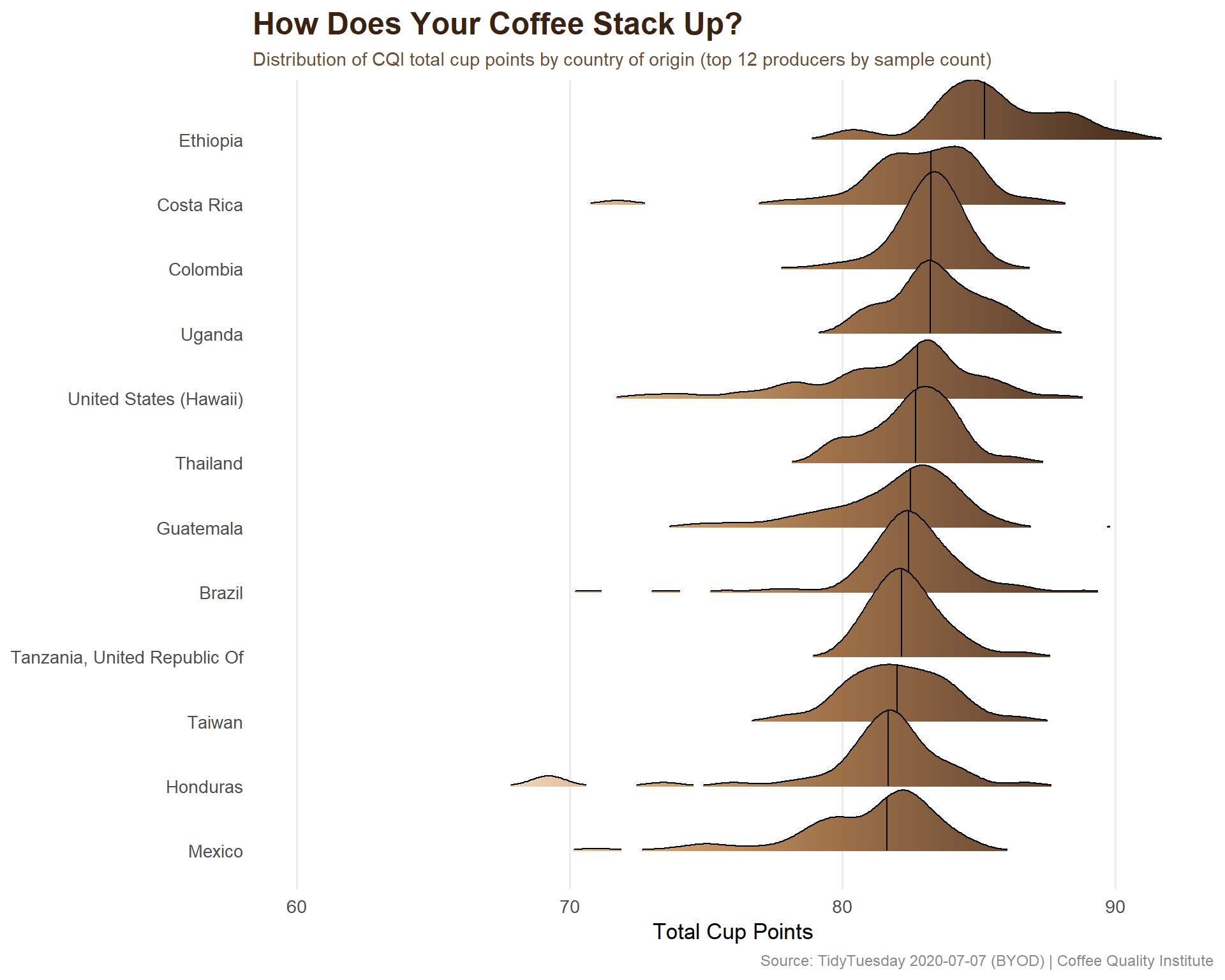
The hero plot shows the distribution of quality scores across the top coffee-producing countries as ridge plots, with a warm coffee-inspired color palette.

# Coffee-inspired palette — light roast to dark roast
coffee_gradient <- c(
  "#F5E6D3",  # cream
  "#D4A574",  # light roast
  "#A0724A",  # medium roast
  "#6F4E37",  # dark roast
  "#3B2314"   # espresso
)

# Get top 12 countries by sample count
top_countries <- coffee %>%
  filter(total_cup_points > 0) %>%
  count(country_of_origin, sort = TRUE) %>%
  head(12) %>%
  pull(country_of_origin)

plot_data <- coffee %>%
  filter(
    country_of_origin %in% top_countries,
    total_cup_points > 50
  ) %>%
  mutate(
    country_of_origin = fct_reorder(country_of_origin, total_cup_points, .fun = median)
  )

# Calculate medians for annotation
country_medians <- plot_data %>%
  group_by(country_of_origin) %>%
  summarize(med = median(total_cup_points), .groups = "drop")

ggplot(plot_data, aes(x = total_cup_points, y = country_of_origin, fill = after_stat(x))) +
  geom_density_ridges_gradient(
    scale = 1.5,
    rel_min_height = 0.01,
    quantile_lines = TRUE,
    quantiles = 2
  ) +
  scale_fill_gradientn(
    colors = coffee_gradient,
    name = "Cup Points"
  ) +
  scale_x_continuous(limits = c(60, 92)) +
  labs(
    title = "How Does Your Coffee Stack Up?",
    subtitle = "Distribution of CQI total cup points by country of origin (top 12 producers by sample count)",
    x = "Total Cup Points",
    y = NULL,
    caption = "Source: TidyTuesday 2020-07-07 (BYOD) | Coffee Quality Institute"
  ) +
  theme_minimal(base_size = 13) +
  theme(
    plot.title = element_text(face = "bold", size = 18, color = "#3B2314"),
    plot.subtitle = element_text(size = 11, color = "#6F4E37"),
    plot.caption = element_text(size = 9, color = "#888888"),
    legend.position = "none",
    panel.grid.minor = element_blank(),
    panel.grid.major.y = element_blank()
  )

Final thoughts and takeaways

The Coffee Quality Institute data reveals a fascinating picture of what drives coffee quality scores. The most immediate finding is how tightly clustered the scores are — most reviewed coffees land between 75 and 88 total cup points, which makes sense given that CQI reviews tend to evaluate specialty-grade coffee that has already passed initial quality screens.

Among the quality attributes, flavor and aftertaste show the highest coefficient of variation, meaning they’re the dimensions where coffees differentiate themselves most. Aroma and body, by contrast, are more consistent across samples. This suggests that if you’re evaluating a coffee, the lingering finish and primary flavor notes are where the real action is.

The altitude-quality correlation, while statistically present, is modest. Higher-altitude farms do tend to produce slightly higher-rated coffees, but altitude alone doesn’t explain the variance nearly as much as origin country and processing method. The coffee industry’s obsession with altitude as a quality signal is somewhat overstated by the data.

Tip

For home coffee enthusiasts: the processing method (washed vs. natural vs. honey) often has a bigger impact on your cup than altitude or even country of origin. If you want to explore flavor differences, try the same origin processed two different ways — it’s the fastest path to understanding what you personally value in a cup.