Tidy Tuesday: Astronomy Picture of the Day

tidytuesday

astronomy

text-analysis

Mining NASA’s APOD archive (2007-2025) — what astronomical subjects capture the most attention, and how has the archive evolved over nearly two decades?

Author

Sean Thimons

Published

January 20, 2026

Preface

From TidyTuesday repository.

The Astronomy Picture of the Day (APOD) archive contains daily astronomy-related images with a scientific explanation, spanning 2007–2025. The data originates from NASA’s popular APOD website and has been curated into the astropic R package.

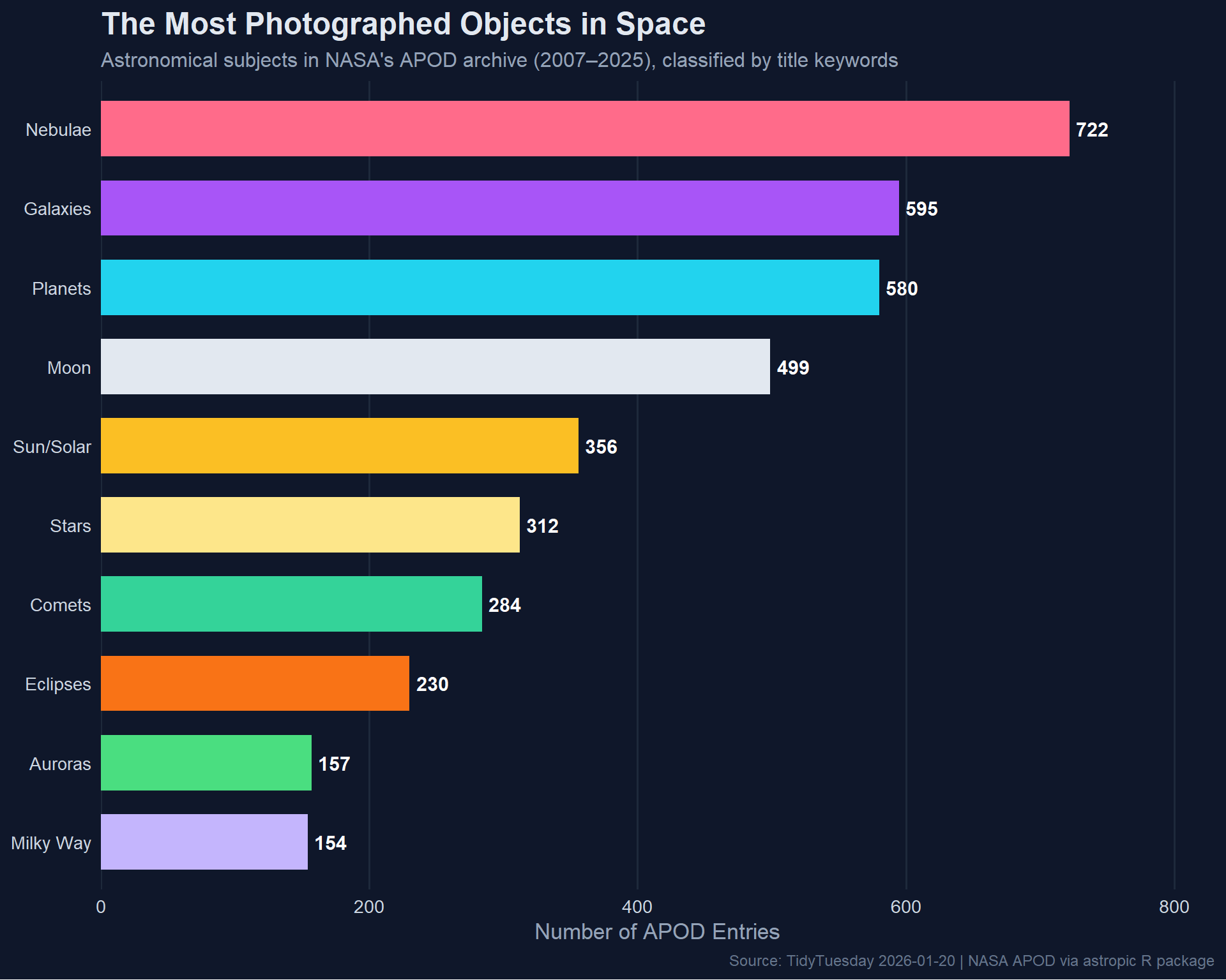
What types of objects are most common in the archive?

Are any images posted more than once?

Loading necessary packages

My handy booster pack that allows me to install (if needed) and load my usual and favorite packages, as well as some helpful functions.

Code

# Packages ----------------------------------------------------------------

{
  if (!requireNamespace("pak", quietly = TRUE)) {
    install.packages(
      "pak",
      repos = sprintf(
        "https://r-lib.github.io/p/pak/stable/%s/%s/%s",
        .Platform$pkgType,
        R.Version()$os,
        R.Version()$arch
      )
    )
  }

  install_booster_pack <- function(package, load = TRUE) {
    for (pkg in package) {
      if (!requireNamespace(pkg, quietly = TRUE)) {
        pak::pkg_install(pkg)
      }
      if (load) {
        library(pkg, character.only = TRUE)
      }
    }
  }

  if (file.exists('packages.txt')) {
    packages <- read.table('packages.txt')
    install_booster_pack(package = packages$Package, load = FALSE)
    rm(packages)
  } else {
    booster_pack <- c(
      ### IO ----
      'fs',
      'here',
      'janitor',
      'rio',
      'tidyverse',

      ### EDA ----
      'skimr',

      ### Text ----
      'tidytext',

      ### Plot ----
      'ggrepel',
      'ggtext',

      ### Misc ----
      'tidytuesdayR'
    )

    install_booster_pack(package = booster_pack, load = TRUE)
    rm(install_booster_pack, booster_pack)
  }

  # Custom Functions ----

  `%ni%` <- Negate(`%in%`)

  geometric_mean <- function(x) {
    exp(mean(log(x[x > 0]), na.rm = TRUE))
  }

  my_skim <- skim_with(
    numeric = sfl(
      n = length,
      min = ~ min(.x, na.rm = T),
      p25 = ~ stats::quantile(., probs = .25, na.rm = TRUE, names = FALSE),
      med = ~ median(.x, na.rm = T),
      p75 = ~ stats::quantile(., probs = .75, na.rm = TRUE, names = FALSE),
      max = ~ max(.x, na.rm = T),
      mean = ~ mean(.x, na.rm = T),
      geo_mean = ~ geometric_mean(.x),
      sd = ~ stats::sd(., na.rm = TRUE),
      hist = ~ inline_hist(., 5)
    ),
    append = FALSE
  )
}

Load raw data from package

raw <- tidytuesdayR::tt_load('2026-01-20')

apod <- raw$apod

Exploratory Data Analysis

The my_skim() function is a modified version of the skimr::skim() function that returns the number of missing data points (cells as NA) as well as the inverse (e.g.: number of rows that are not NA), the count, minimum, 25%, median, 75%, max, mean, geometric mean, and standard deviation. It also generates a little ASCII histogram. Neat!

APOD Archive

I’ll drop the URL columns and explanation text for the initial skim — they’re useful later but not for profiling.

apod %>%
  select(-url, -hdurl, -explanation) %>%
  my_skim(.)

Data summary
Name	Piped data
Number of rows	6888
Number of columns	4
_______________________
Column type frequency:
character	3
Date	1
________________________
Group variables	None

Variable type: character

skim_variable	n_missing	complete_rate	min	max	n_unique
copyright	2699	0.61	3	160	2251
media_type	0	1.00	5	5	3
title	0	1.00	4	66	5151

Variable type: Date

skim_variable	n_missing	complete_rate	min	max	median	n_unique
date	0	1	2007-01-01	2025-12-23	2016-06-28	6888

apod %>%
  count(media_type, sort = TRUE)

# A tibble: 3 × 2
  media_type     n
  <chr>      <int>
1 image       6499
2 video        379
3 other         10

Date Coverage

apod %>%
  mutate(year = year(date)) %>%
  count(year) %>%
  print(n = 30)

# A tibble: 19 × 2
    year     n
   <dbl> <int>
 1  2007   363
 2  2008   365
 3  2009   361
 4  2010   357
 5  2011   361
 6  2012   364
 7  2013   365
 8  2014   363
 9  2015   365
10  2016   366
11  2017   365
12  2018   364
13  2019   365
14  2020   365
15  2021   365
16  2022   365
17  2023   365
18  2024   366
19  2025   338

APOD Archive Analysis

Duplicate Images

The repo asks: are any images posted more than once? Let’s check for repeated URLs and titles.

# Check for duplicate URLs
apod %>%
  filter(!is.na(url)) %>%
  count(url, sort = TRUE) %>%
  filter(n > 1) %>%
  head(10)

# A tibble: 10 × 2
   url                                                                         n
   <chr>                                                                   <int>
 1 https://www.youtube.com/embed/OfM7VlonD5c?rel=0                             4
 2 https://www.youtube.com/embed/sNUNB6CMnE8?rel=0                             4
 3 //player.vimeo.com/video/108650530?title=0&byline=0&portrait=0&badge=0…     3
 4 https://apod.nasa.gov/apod/image/1803/AstroSoM/hudf.html                    3
 5 https://player.vimeo.com/video/32095756?title=0&byline=0&portrait=0         3
 6 https://www.youtube.com/embed/B1R3dTdcpSU?rel=0                             3
 7 https://www.youtube.com/embed/FG0fTKAqZ5g?rel=0                             3
 8 https://www.youtube.com/embed/I_88S8DWbcU?rel=0                             3
 9 https://www.youtube.com/embed/PBL1RBj-P1g?rel=0                             3
10 https://www.youtube.com/embed/afHfMMC-MJE?rel=0                             3

# Check for duplicate titles
apod %>%
  count(title, sort = TRUE) %>%
  filter(n > 1) %>%
  head(15)

# A tibble: 15 × 2
   title                                           n
   <chr>                                       <int>
 1 M31: The Andromeda Galaxy                      10
 2 The Horsehead Nebula                           10
 3 M13: The Great Globular Cluster in Hercules     9
 4 NGC 4565: Galaxy on Edge                        9
 5 NGC 602 and Beyond                              8
 6 The Medusa Nebula                               8
 7 The Seagull Nebula                              8
 8 A Beautiful Trifid                              7
 9 Galaxies in the River                           7
10 Halo of the Cat's Eye                           7
11 Lynds Dark Nebula 1251                          7
12 M1: The Crab Nebula from Hubble                 7
13 M27: The Dumbbell Nebula                        7
14 M45: The Pleiades Star Cluster                  7
15 Millions of Stars in Omega Centauri             7

Most Common Subjects via Title Keywords

To answer “what types of objects are most common,” we can tokenize the titles and look for astronomical keywords.

# Define astronomical object categories
astro_keywords <- tribble(
  ~keyword, ~category,
  "nebula", "Nebulae",
  "galaxy", "Galaxies",
  "moon", "Moon",
  "sun", "Sun/Solar",
  "solar", "Sun/Solar",
  "eclipse", "Eclipses",
  "mars", "Planets",
  "jupiter", "Planets",
  "saturn", "Planets",
  "venus", "Planets",
  "mercury", "Planets",
  "comet", "Comets",
  "aurora", "Auroras",
  "milky way", "Milky Way",
  "meteor", "Meteors",
  "supernova", "Supernovae",
  "cluster", "Star Clusters",
  "star", "Stars"
)

# Tokenize titles and match keywords
title_words <- apod %>%
  select(date, title) %>%
  mutate(title_lower = str_to_lower(title))

# Count keyword matches
keyword_counts <- astro_keywords %>%
  rowwise() %>%
  mutate(
    count = sum(str_detect(title_words$title_lower, keyword))
  ) %>%
  ungroup() %>%
  group_by(category) %>%
  summarize(count = sum(count), .groups = "drop") %>%
  arrange(desc(count))

keyword_counts

# A tibble: 13 × 2
   category      count
   <chr>         <int>
 1 Planets         772
 2 Nebulae         722
 3 Stars           548
 4 Moon            538
 5 Sun/Solar       487
 6 Galaxies        472
 7 Comets          311
 8 Eclipses        230
 9 Star Clusters   206
10 Milky Way       180
11 Auroras         157
12 Meteors         120
13 Supernovae       88

Trends Over Time

How has the mix of subjects changed year by year?

# Tag each APOD entry with a category (first match wins)
apod_tagged <- apod %>%
  mutate(
    title_lower = str_to_lower(title),
    category = case_when(
      str_detect(title_lower, "nebula") ~ "Nebulae",
      str_detect(title_lower, "galaxy|galaxies") ~ "Galaxies",
      str_detect(title_lower, "eclipse") ~ "Eclipses",
      str_detect(title_lower, "aurora") ~ "Auroras",
      str_detect(title_lower, "comet") ~ "Comets",
      str_detect(title_lower, "moon") ~ "Moon",
      str_detect(title_lower, "sun|solar") ~ "Sun/Solar",
      str_detect(title_lower, "mars|jupiter|saturn|venus|mercury") ~ "Planets",
      str_detect(title_lower, "milky way") ~ "Milky Way",
      str_detect(title_lower, "meteor") ~ "Meteors",
      str_detect(title_lower, "cluster") ~ "Star Clusters",
      str_detect(title_lower, "star") ~ "Stars",
      TRUE ~ "Other"
    ),
    year = year(date)
  )

apod_tagged %>%
  filter(category != "Other") %>%
  count(year, category) %>%
  pivot_wider(names_from = category, values_from = n, values_fill = 0) %>%
  head(20)

# A tibble: 19 × 13
    year Auroras Comets Eclipses Galaxies Meteors `Milky Way`  Moon Nebulae
   <dbl>   <int>  <int>    <int>    <int>   <int>       <int> <int>   <int>
 1  2007       4     27       11       28       1           3    28      40
 2  2008       4      8        8       31       2           7    19      35
 3  2009       4      8        7       31       6           9    29      42
 4  2010       6      8       14       32       5           9    24      25
 5  2011       6     13       12       31       3           6    16      31
 6  2012      14      5        9       26       3           9    32      42
 7  2013      11     27       10       25      10           6    23      34
 8  2014      13     18       11       29       0           8    26      43
 9  2015      15     19       13       35       1          14    24      26
10  2016      10     11       10       36       2          10    25      43
11  2017       8     11       23       31       5           7    20      37
12  2018       7      8       12       26       4           9    28      43
13  2019       4      5       13       40       2           9    26      38
14  2020       3     20       10       28       6           9    30      32
15  2021      10     16       16       27       6           5    26      35
16  2022       7     12       11       32       3          10    36      44
17  2023      13     17       14       42       3          10    32      49
18  2024      16     30       17       32       7           8    32      43
19  2025       2     21        9       33       4           6    23      40
# ℹ 4 more variables: Planets <int>, `Star Clusters` <int>, Stars <int>,
#   `Sun/Solar` <int>

Visualizing the APOD Universe

The hero plot shows the most common astronomical subjects across the archive, styled with a deep-space aesthetic.

# Space-themed palette
space_cols <- c(
  "Nebulae" = "#FF6B8A",
  "Galaxies" = "#A855F7",
  "Moon" = "#E2E8F0",
  "Sun/Solar" = "#FBBF24",
  "Eclipses" = "#F97316",
  "Planets" = "#22D3EE",
  "Comets" = "#34D399",
  "Auroras" = "#4ADE80",
  "Milky Way" = "#C4B5FD",
  "Meteors" = "#FB923C",
  "Stars" = "#FDE68A",
  "Supernovae" = "#F43F5E",
  "Star Clusters" = "#818CF8"
)

# Prepare data — top categories by total count
top_categories <- apod_tagged %>%
  filter(category != "Other") %>%
  count(category, sort = TRUE) %>%
  head(10)

ggplot(top_categories, aes(x = reorder(category, n), y = n, fill = category)) +
  geom_col(width = 0.7, show.legend = FALSE) +
  geom_text(
    aes(label = n),
    hjust = -0.2,
    color = "white",
    fontface = "bold",
    size = 4
  ) +
  scale_fill_manual(values = space_cols) +
  scale_y_continuous(expand = expansion(mult = c(0, 0.15))) +
  coord_flip() +
  labs(
    title = "The Most Photographed Objects in Space",
    subtitle = "Astronomical subjects in NASA's APOD archive (2007\u20132025), classified by title keywords",
    x = NULL,
    y = "Number of APOD Entries",
    caption = "Source: TidyTuesday 2026-01-20 | NASA APOD via astropic R package"
  ) +
  theme_minimal(base_size = 13) +
  theme(
    plot.background = element_rect(fill = "#0F172A", color = NA),
    panel.background = element_rect(fill = "#0F172A", color = NA),
    text = element_text(color = "white"),
    plot.title = element_text(face = "bold", size = 18, color = "#E2E8F0"),
    plot.subtitle = element_text(size = 12, color = "#94A3B8"),
    plot.caption = element_text(size = 9, color = "#64748B"),
    axis.text = element_text(color = "#CBD5E1"),
    axis.title = element_text(color = "#94A3B8"),
    panel.grid.major.y = element_blank(),
    panel.grid.major.x = element_line(color = "#1E293B"),
    panel.grid.minor = element_blank()
  )

Final thoughts and takeaways

NASA’s Astronomy Picture of the Day is one of the longest-running and most beloved science communication projects on the internet. This archive spanning nearly two decades reveals what captures our collective astronomical imagination — and nebulae consistently come out on top, which makes sense given their visual drama and the stunning images that space telescopes produce.

Galaxies and our own Moon round out the top three, reflecting both the accessibility of lunar photography for amateur astronomers and the deep fascination with the large-scale structure of the universe. The presence of auroras and eclipses in the rankings highlights how APOD balances deep-sky objects with phenomena visible from Earth, keeping the archive grounded (literally) for a general audience.

The duplicate analysis reveals that some iconic images do get revisited — either because the same event is captured from different perspectives or because a particularly striking image merits a re-share. This isn’t noise; it’s editorial curation at work.

Tip

The title-keyword approach to classification is deliberately simple. A more sophisticated analysis could use NLP on the explanation text to capture objects mentioned in the description but not the title. The explanations are rich with scientific context that the titles alone don’t capture.