Tidy Tuesday: The 2026 Winter Olympics

tidytuesday
R
sports
olympics
geography
Mapping the geographic pulse of the Milano-Cortina 2026 Winter Olympics — how 1,866 events spread across 13 venues and 6 host cities over 19 days.
Author

Sean Thimons

Published

February 12, 2026

Preface

From TidyTuesday repository.

This week’s dataset focuses on the Milano-Cortina 2026 Winter Olympics schedule. The data contains 1,866 Olympic events including competition and training sessions across 16 winter sports disciplines. The schedule spans February 4–22, 2026 and features timezone conversions, venue details, and medal event classifications.

Loading necessary packages

My handy booster pack that allows me to install (if needed) and load my usual and favorite packages, as well as some helpful functions.

Code
# Packages ----------------------------------------------------------------

{
  # Install pak if it's not already installed
  if (!requireNamespace("pak", quietly = TRUE)) {
    install.packages(
      "pak",
      repos = sprintf(
        "https://r-lib.github.io/p/pak/stable/%s/%s/%s",
        .Platform$pkgType,
        R.Version()$os,
        R.Version()$arch
      )
    )
  }

  # CRAN Packages ----
  install_booster_pack <- function(package, load = TRUE) {
    for (pkg in package) {
      if (!requireNamespace(pkg, quietly = TRUE)) {
        pak::pkg_install(pkg)
      }
      if (load) {
        library(pkg, character.only = TRUE)
      }
    }
  }

  if (file.exists('packages.txt')) {
    packages <- read.table('packages.txt')

    install_booster_pack(package = packages$Package, load = FALSE)

    rm(packages)
  } else {
    ## Packages ----

    booster_pack <- c(
      ### IO ----
      'fs',
      'here',
      'janitor',
      'rio',
      'tidyverse',

      ### EDA ----
      'skimr',

      ### Plot ----
      'paletteer',
      'patchwork',
      'ggtext',
      'ggrepel',

      ### Reporting ----
      'gt',

      ### Misc ----
      'tidytuesdayR'
    )

    # ! Change load flag to load packages
    install_booster_pack(package = booster_pack, load = TRUE)
    rm(install_booster_pack, booster_pack)
  }

  # Custom Functions ----

  `%ni%` <- Negate(`%in%`)

  geometric_mean <- function(x) {
    exp(mean(log(x[x > 0]), na.rm = TRUE))
  }

  my_skim <- skim_with(
    numeric = sfl(
      n = length,
      min = ~ min(.x, na.rm = T),
      p25 = ~ stats::quantile(., probs = .25, na.rm = TRUE, names = FALSE),
      med = ~ median(.x, na.rm = T),
      p75 = ~ stats::quantile(., probs = .75, na.rm = TRUE, names = FALSE),
      max = ~ max(.x, na.rm = T),
      mean = ~ mean(.x, na.rm = T),
      geo_mean = ~ geometric_mean(.x),
      sd = ~ stats::sd(., na.rm = TRUE),
      hist = ~ inline_hist(., 5)
    ),
    append = FALSE
  )
}

Load raw data from package

raw <- tidytuesdayR::tt_load('2026-02-10')

schedule <- raw$schedule %>%
  clean_names() %>%
  mutate(
    date = as.Date(date),
    is_medal_event = as.logical(is_medal_event),
    is_training = as.logical(is_training),
    estimated_start = as.logical(estimated_start),
    start_datetime_local = as.POSIXct(start_datetime_local),
    end_datetime_local = as.POSIXct(end_datetime_local),
    start_datetime_utc = as.POSIXct(start_datetime_utc, tz = "UTC"),
    end_datetime_utc = as.POSIXct(end_datetime_utc, tz = "UTC")
  )

Exploratory Data Analysis

The my_skim() function is a modified version of the skimr::skim() function that returns the number of missing data points (cells as NA) as well as the inverse (e.g.: number of rows that are not NA), the count, minimum, 25%, median, 75%, max, mean, geometric mean, and standard deviation. It also generates a little ASCII histogram. Neat!

Schedule overview

schedule %>%
  select(
    -session_code,
    -event_code,
    -discipline_code,
    -venue_code,
    -venue_slug,
    -location_code,
    -start_datetime_utc,
    -end_datetime_utc
  ) %>%
  my_skim()
Data summary
Name Piped data
Number of rows 1866
Number of columns 13
_______________________
Column type frequency:
character 5
Date 1
difftime 2
logical 3
POSIXct 2
________________________
Group variables None

Variable type: character

skim_variable n_missing complete_rate min max empty n_unique whitespace
discipline_name 0 1.00 4 25 0 16 0
event_description 0 1.00 10 40 0 477 0
venue_name 63 0.97 17 35 0 13 0
location_name 0 1.00 17 30 0 30 0
day_of_week 0 1.00 6 9 0 7 0

Variable type: Date

skim_variable n_missing complete_rate min max median n_unique
date 0 1 2026-02-04 2026-02-22 2026-02-13 19

Variable type: difftime

skim_variable n_missing complete_rate min max median n_unique
start_time 0 1 28800 secs 81240 secs 51300 secs 186
end_time 0 1 29880 secs 85200 secs 57240 secs 254

Variable type: logical

skim_variable n_missing complete_rate mean count
is_medal_event 0 1 0.18 FAL: 1522, TRU: 344
is_training 0 1 0.13 FAL: 1620, TRU: 246
estimated_start 0 1 0.00 FAL: 1861, TRU: 5

Variable type: POSIXct

skim_variable n_missing complete_rate min max median n_unique
start_datetime_local 0 1 2026-02-04 11:30:00 2026-02-22 14:10:00 2026-02-13 19:00:00 487
end_datetime_local 0 1 2026-02-04 13:30:00 2026-02-22 16:40:00 2026-02-13 20:24:10 509

The schedule contains 1866 total events across 16 disciplines and 14 venues. Events span from 2026-02-04 to 2026-02-22 — a 19-day window that includes both training and competition sessions.

Key observations from the skim:

  • Training vs. competition: 246 training sessions and 1620 competition events
  • Medal events: 344 medal sessions out of the full schedule
  • Venue concentration: Some venues host hundreds of events (Cortina Curling Olympic Stadium alone accounts for a huge share), while others are more specialized

Host city extraction

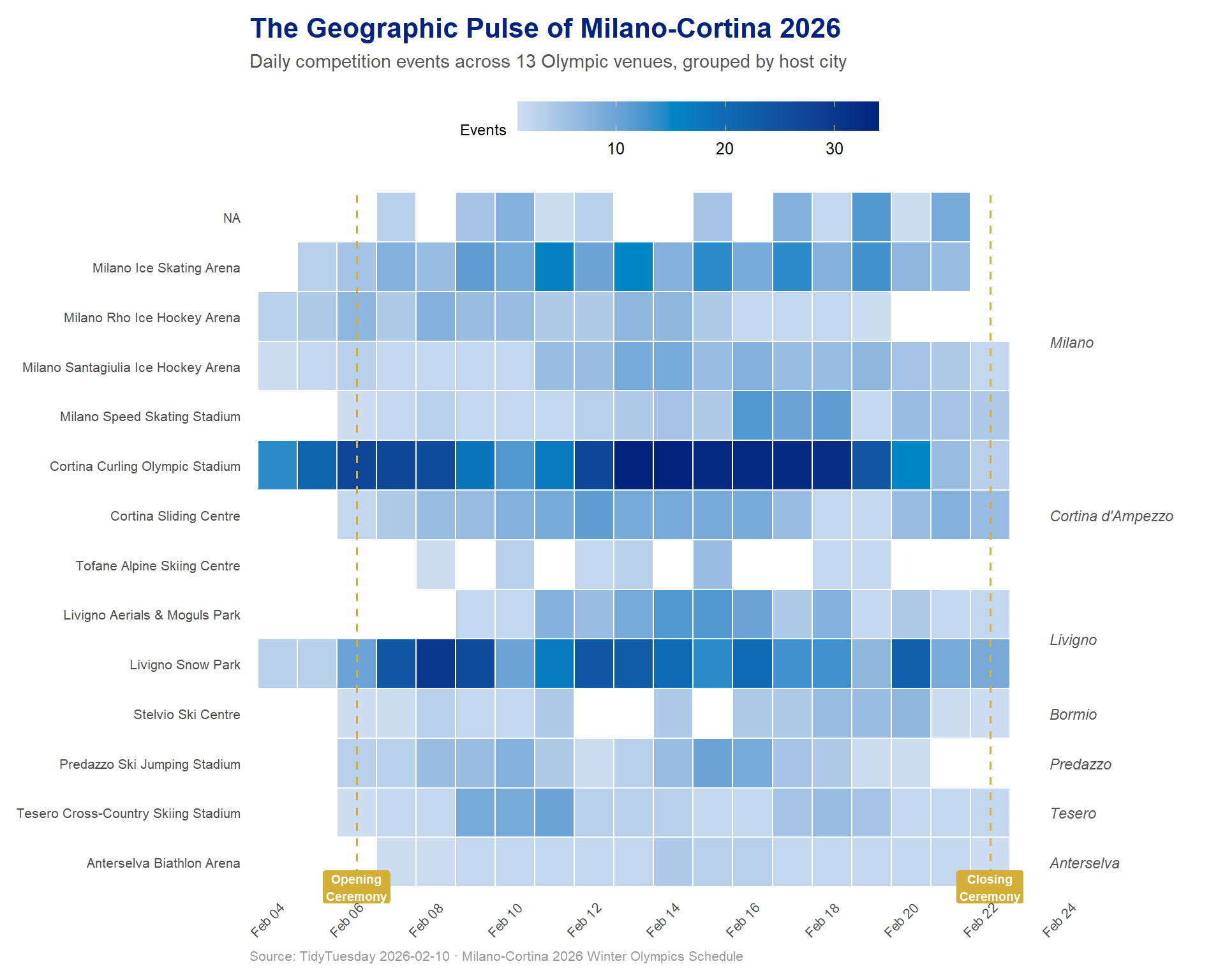
The 2026 Games are uniquely distributed across northern Italy. Let’s extract the host city from each venue name and see how the Games are geographically structured.

schedule <- schedule %>%
  mutate(
    host_city = case_when(
      str_detect(venue_name, "^Milano") ~ "Milano",
      str_detect(venue_name, "^Cortina") ~ "Cortina d'Ampezzo",
      str_detect(venue_name, "^Livigno") ~ "Livigno",
      str_detect(venue_name, "^Predazzo") ~ "Predazzo",
      str_detect(venue_name, "^Tesero") ~ "Tesero",
      str_detect(venue_name, "^Anterselva") ~ "Anterselva",
      str_detect(venue_name, "^Stelvio") ~ "Bormio",
      str_detect(venue_name, "^Tofane") ~ "Cortina d'Ampezzo",
      TRUE ~ "Other"
    )
  )

schedule %>%
  filter(!is_training) %>%
  count(host_city, sort = TRUE) %>%
  mutate(pct = scales::percent(n / sum(n))) %>%
  gt() %>%
  cols_label(
    host_city = "Host City",
    n = "Competition Events",
    pct = "Share"
  ) %>%
  tab_header(title = "Competition events by host city")
Competition events by host city
Host City Competition Events Share
Cortina d'Ampezzo 567 35.00%
Milano 399 24.63%
Livigno 380 23.46%
Predazzo 70 4.32%
Tesero 68 4.20%
Other 57 3.52%
Bormio 46 2.84%
Anterselva 33 2.04%
NoteA distributed Games

Unlike many Winter Olympics concentrated in a single mountain region, Milano-Cortina 2026 spreads across the Italian Alps and into the Po Valley. Milano hosts the ice sports (figure skating, speed skating, short track, hockey), while the mountain towns — Cortina, Livigno, Bormio — handle the snow and sliding disciplines. This geographic spread is a defining feature of these Games.

Venue Geography Analysis

Disciplines per venue

Each venue is purpose-built or adapted for specific sports. Let’s map which disciplines live where.

venue_disciplines <- schedule %>%
  filter(!is_training) %>%
  count(venue_name, host_city, discipline_name, sort = TRUE)

venue_disciplines %>%
  group_by(venue_name, host_city) %>%
  summarise(
    disciplines = paste(discipline_name, collapse = ", "),
    total_events = sum(n),
    .groups = "drop"
  ) %>%
  arrange(desc(total_events)) %>%
  gt() %>%
  cols_label(
    venue_name = "Venue",
    host_city = "City",
    disciplines = "Disciplines",
    total_events = "Events"
  ) %>%
  tab_header(title = "Venue utilization and discipline mapping")
Venue utilization and discipline mapping
Venue City Disciplines Events
Cortina Curling Olympic Stadium Cortina d'Ampezzo Curling 436
Livigno Snow Park Livigno Snowboard, Freestyle Skiing 297
Milano Ice Skating Arena Milano Short Track Speed Skating, Figure Skating 162
Cortina Sliding Centre Cortina d'Ampezzo Bobsleigh, Luge, Skeleton 112
Milano Santagiulia Ice Hockey Arena Milano Ice Hockey 88
Livigno Aerials & Moguls Park Livigno Freestyle Skiing 83
Milano Speed Skating Stadium Milano Speed Skating 78
Milano Rho Ice Hockey Arena Milano Ice Hockey 71
Predazzo Ski Jumping Stadium Predazzo Ski Jumping, Nordic Combined 70
Tesero Cross-Country Skiing Stadium Tesero Cross-Country Skiing, Nordic Combined 68
NA Other Freestyle Skiing, Ice Hockey, Nordic Combined, Alpine Skiing 57
Stelvio Ski Centre Bormio Alpine Skiing, Ski Mountaineering 46
Anterselva Biathlon Arena Anterselva Biathlon 33
Tofane Alpine Skiing Centre Cortina d'Ampezzo Alpine Skiing 19

Medal density by venue

Not all events are created equal. Some venues host dozens of rounds leading to a handful of medal moments; others are medal-dense. The medal density — the share of competition events that award medals — reveals which venues are built for the climactic moments.

venue_medal_density <- schedule %>%
  filter(!is_training) %>%
  group_by(venue_name, host_city) %>%
  summarise(
    total_events = n(),
    medal_events = sum(is_medal_event),
    medal_density = medal_events / total_events,
    .groups = "drop"
  ) %>%
  arrange(desc(medal_density))

venue_medal_density %>%
  mutate(medal_density = scales::percent(medal_density, accuracy = 0.1)) %>%
  gt() %>%
  cols_label(
    venue_name = "Venue",
    host_city = "City",
    total_events = "Total Events",
    medal_events = "Medal Events",
    medal_density = "Medal Density"
  ) %>%
  tab_header(title = "Medal density across Olympic venues")
Medal density across Olympic venues
Venue City Total Events Medal Events Medal Density
Anterselva Biathlon Arena Anterselva 33 33 100.0%
Tesero Cross-Country Skiing Stadium Tesero 68 44 64.7%
Tofane Alpine Skiing Centre Cortina d'Ampezzo 19 12 63.2%
Milano Speed Skating Stadium Milano 78 42 53.8%
Stelvio Ski Centre Bormio 46 24 52.2%
Cortina Sliding Centre Cortina d'Ampezzo 112 35 31.2%
Milano Ice Skating Arena Milano 162 42 25.9%
Predazzo Ski Jumping Stadium Predazzo 70 18 25.7%
NA Other 57 14 24.6%
Livigno Aerials & Moguls Park Livigno 83 18 21.7%
Livigno Snow Park Livigno 297 50 16.8%
Milano Santagiulia Ice Hockey Arena Milano 88 4 4.5%
Cortina Curling Olympic Stadium Cortina d'Ampezzo 436 8 1.8%
Milano Rho Ice Hockey Arena Milano 71 0 0.0%
ImportantCurling: the endurance sport of scheduling

Cortina Curling Olympic Stadium hosts a staggering 436 competition events — more than double any other venue — yet produces only 8 medal sessions (a medal density under 2%). Curling’s round-robin format demands this marathon of matches, making it the most venue-intensive discipline by far.
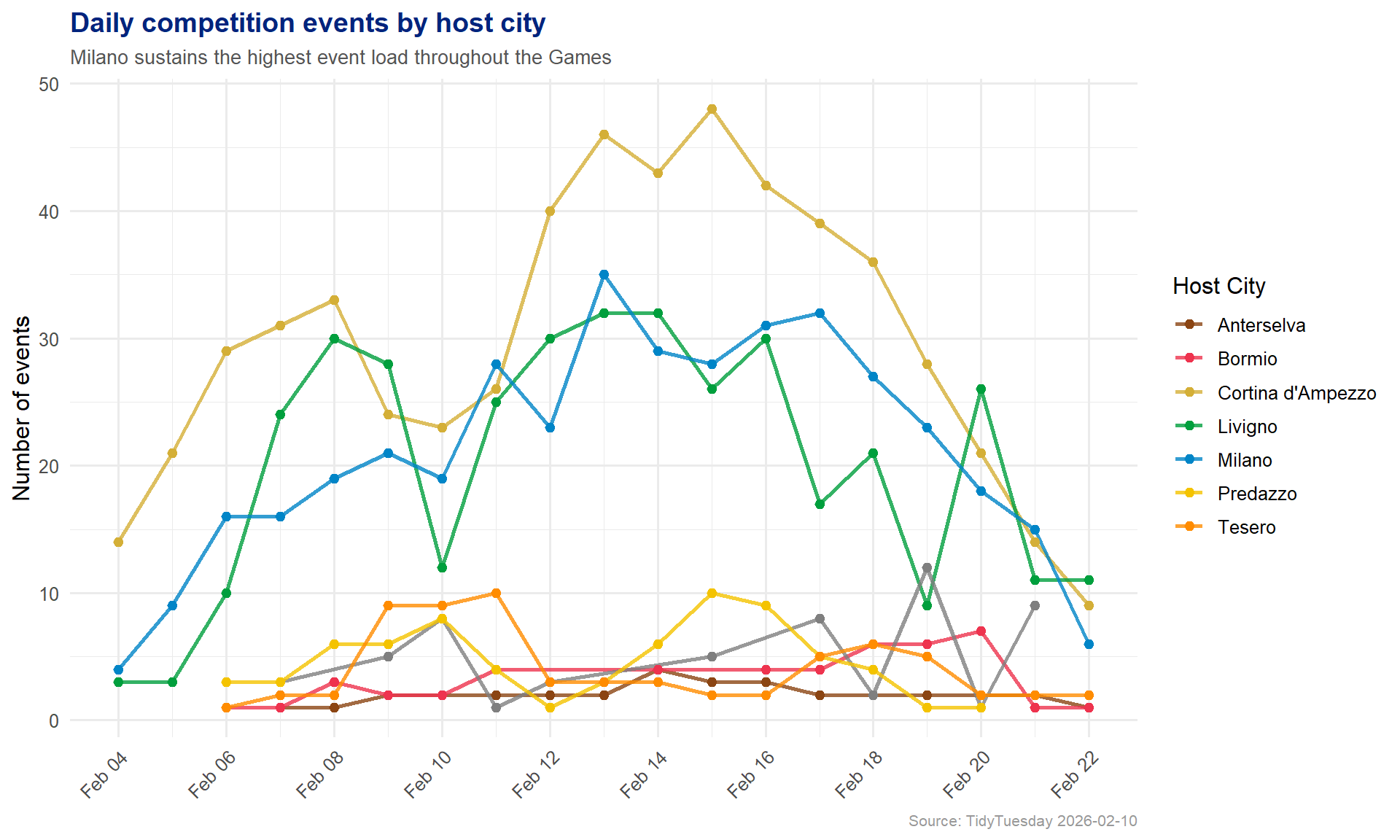
Daily venue activity

daily_venue <- schedule %>%
  filter(!is_training) %>%
  count(date, venue_name, host_city, name = "events")

# Create ordered factor for venues grouped by city
venue_order <- schedule %>%
  filter(!is_training) %>%
  mutate(
    city_order = factor(
      host_city,
      levels = c(
        "Milano",
        "Cortina d'Ampezzo",
        "Livigno",
        "Bormio",
        "Predazzo",
        "Tesero",
        "Anterselva"
      )
    )
  ) %>%
  arrange(city_order, venue_name) %>%
  pull(venue_name) %>%
  unique()

daily_venue <- daily_venue %>%
  mutate(venue_name = factor(venue_name, levels = rev(venue_order)))
# Olympic-inspired color palette
olympic_gradient <- c("#FFFFFF", "#0085C7", "#00247D")

# Key ceremony dates
ceremonies <- tibble(
  date = as.Date(c("2026-02-06", "2026-02-22")),
  label = c("Opening\nCeremony", "Closing\nCeremony")
)

# City labels for venue grouping
city_labels <- daily_venue %>%
  distinct(venue_name, host_city) %>%
  mutate(
    venue_name = factor(venue_name, levels = levels(daily_venue$venue_name))
  ) %>%
  group_by(host_city) %>%
  summarise(
    y_pos = mean(as.numeric(venue_name)),
    .groups = "drop"
  )

# Build the heatmap
p <- ggplot(daily_venue, aes(x = date, y = venue_name, fill = events)) +
  geom_tile(color = "white", linewidth = 0.4) +
  scale_fill_gradient2(
    low = "#FFFFFF",
    mid = "#0085C7",
    high = "#00247D",
    midpoint = 15,
    name = "Events",
    na.value = "#F5F5F5"
  ) +
  scale_x_date(
    date_breaks = "2 days",
    date_labels = "%b %d",
    expand = expansion(mult = c(0.01, 0.05))
  ) +
  # Opening & closing ceremony markers
  geom_vline(
    data = ceremonies,
    aes(xintercept = date),
    linetype = "dashed",
    color = "#D4AF37",
    linewidth = 0.6
  ) +
  geom_label(
    data = ceremonies,
    aes(x = date, y = 0.5, label = label),
    inherit.aes = FALSE,
    fill = "#D4AF37",
    color = "white",
    fontface = "bold",
    size = 2.5,
    label.padding = unit(0.2, "lines"),
    label.size = 0
  ) +
  # City group annotations on the right
  annotate(
    "text",
    x = max(daily_venue$date) + 1.5,
    y = city_labels$y_pos,
    label = city_labels$host_city,
    hjust = 0,
    fontface = "italic",
    size = 3,
    color = "#555555"
  ) +
  coord_cartesian(clip = "off") +
  labs(
    title = "The Geographic Pulse of Milano-Cortina 2026",
    subtitle = "Daily competition events across 13 Olympic venues, grouped by host city",
    x = NULL,
    y = NULL,
    caption = "Source: TidyTuesday 2026-02-10 · Milano-Cortina 2026 Winter Olympics Schedule"
  ) +
  theme_minimal(base_size = 12) +
  theme(
    plot.title = element_text(face = "bold", size = 16, color = "#00247D"),
    plot.subtitle = element_text(
      size = 11,
      color = "#555555",
      margin = margin(b = 12)
    ),
    plot.caption = element_text(size = 8, color = "#999999", hjust = 0),
    axis.text.y = element_text(size = 8),
    axis.text.x = element_text(size = 8, angle = 45, hjust = 1),
    legend.position = "top",
    legend.title = element_text(size = 9),
    legend.key.width = unit(1.5, "cm"),
    panel.grid = element_blank(),
    plot.margin = margin(10, 80, 10, 10)
  )

p

Venue activity over time by city

city_daily <- schedule %>%
  filter(!is_training) %>%
  count(date, host_city, name = "events")

city_colors <- c(
  "Milano" = "#0085C7",
  "Cortina d'Ampezzo" = "#D4AF37",
  "Livigno" = "#009F3D",
  "Bormio" = "#EE334E",
  "Predazzo" = "#F4C300",
  "Tesero" = "#FF8C00",
  "Anterselva" = "#8B4513"
)

ggplot(city_daily, aes(x = date, y = events, color = host_city)) +
  geom_line(linewidth = 1, alpha = 0.8) +
  geom_point(size = 2) +
  scale_color_manual(values = city_colors, name = "Host City") +
  scale_x_date(date_breaks = "2 days", date_labels = "%b %d") +
  labs(
    title = "Daily competition events by host city",
    subtitle = "Milano sustains the highest event load throughout the Games",
    x = NULL,
    y = "Number of events",
    caption = "Source: TidyTuesday 2026-02-10"
  ) +
  theme_minimal(base_size = 12) +
  theme(
    plot.title = element_text(face = "bold", size = 14, color = "#00247D"),
    plot.subtitle = element_text(size = 10, color = "#555555"),
    plot.caption = element_text(size = 8, color = "#999999"),
    axis.text.x = element_text(angle = 45, hjust = 1),
    legend.position = "right"
  )

Final thoughts and takeaways

The Milano-Cortina 2026 Winter Olympics are architecturally unique: rather than clustering events in a single alpine basin, these Games sprawl across the Italian Alps and down into the Po Valley. This analysis reveals several patterns in that geographic design:

Milano is the engine room. With four venues hosting ice sports — figure skating, short track, speed skating, and two hockey arenas — Milano sustains the highest daily event count throughout the Games. The city’s venues are active nearly every day from opening to closing ceremony.

Cortina’s curling dominance is deceptive. The Cortina Curling Olympic Stadium generates by far the most events of any venue, but its medal density is vanishingly low. The round-robin format means hundreds of sessions build to just a handful of medal moments — a sharp contrast to venues like the speed skating stadium or biathlon arena where a larger share of events produce medals.

Mountain venues are specialists. The alpine and Nordic venues — Bormio, Predazzo, Tesero, Anterselva — each host one or two disciplines and operate on tighter, more concentrated schedules. Their activity windows are shorter but intense.

The mid-Games peak is universal. Across nearly every venue, event density peaks around February 13–16, suggesting a deliberate scheduling strategy that builds momentum through the first week and then ramps into a climactic stretch before the closing ceremonies.

This geographic distribution presents both logistical challenges (athlete transport, spectator travel between cities separated by hours of mountain driving) and opportunities (multiple cities share the economic and cultural benefits of hosting). Whether this distributed model becomes a template for future Games remains to be seen.