Tidy Tuesday: Agricultural Production Statistics in New Zealand

New Zealand’s agriculture has transformed over 90 years — sheep once outnumbered people 22-to-1 at the 1982 peak. What happened next reveals an entire economy in transition.

Preface

From the TidyTuesday repository.

This dataset examines agricultural production statistics from New Zealand, compiled by StatsNZ. The analysis explores trends in various agricultural sectors, particularly noting the decline in the sheep-to-people ratio from a peak of 22 sheep per person in the 1980s to approximately 4.5 sheep per person currently.

Suggested questions: Does sheep production show a unique decline pattern compared to other meat industries? Which agricultural sectors have experienced the most significant production growth?

Loading necessary packages

My handy booster pack that allows me to install (if needed) and load my usual and favorite packages, as well as some helpful functions.

# Packages ----------------------------------------------------------------

{
  # Install pak if it's not already installed
  if (!requireNamespace("pak", quietly = TRUE)) {
    install.packages(
      "pak",
      repos = sprintf(
        "https://r-lib.github.io/p/pak/stable/%s/%s/%s",
        .Platform$pkgType,
        R.Version()$os,
        R.Version()$arch
      )
    )
  }

  # CRAN Packages ----
  install_booster_pack <- function(package, load = TRUE) {
    for (pkg in package) {
      if (!requireNamespace(pkg, quietly = TRUE)) {
        pak::pkg_install(pkg)
      }
      if (load) {
        library(pkg, character.only = TRUE)
      }
    }
  }

  booster_pack <- c(
    ### IO ----
    'fs',
    'here',
    'janitor',
    'rio',
    'tidyverse',

    ### EDA ----
    'skimr',

    ### Plot ----
    'paletteer',          # Color palette collection
    'ggrepel',            # Non-overlapping labels
    'ggtext',             # Rich text in ggplot

    ### Misc ----
    'tidytuesdayR'
  )

  install_booster_pack(package = booster_pack, load = TRUE)
  rm(install_booster_pack, booster_pack)

  # Custom Functions ----

  `%ni%` <- Negate(`%in%`)

  geometric_mean <- function(x) {
    exp(mean(log(x[x > 0]), na.rm = TRUE))
  }

  my_skim <- skim_with(
    numeric = sfl(
      n = length,
      min = ~ min(.x, na.rm = T),
      p25 = ~ stats::quantile(., probs = .25, na.rm = TRUE, names = FALSE),
      med = ~ median(.x, na.rm = T),
      p75 = ~ stats::quantile(., probs = .75, na.rm = TRUE, names = FALSE),
      max = ~ max(.x, na.rm = T),
      mean = ~ mean(.x, na.rm = T),
      geo_mean = ~ geometric_mean(.x),
      sd = ~ stats::sd(., na.rm = TRUE),
      hist = ~ inline_hist(., 5)
    ),
    append = FALSE
  )
}

Load raw data from package

raw <- tidytuesdayR::tt_load('2026-02-17')

dataset <- raw$dataset %>%
  janitor::clean_names()

Exploratory Data Analysis

The my_skim() function is a modified version of the skimr::skim() function that returns the number of missing data points (cells as NA) as well as the inverse, the count, minimum, 25%, median, 75%, max, mean, geometric mean, and standard deviation. It also generates a little ASCII histogram. Neat!

Agricultural Production Dataset

# Drop free-text label columns before skimming numeric structure
dataset %>%
  select(year_ended_june, value) %>%
  my_skim()

Data summary

Name	Piped data
Number of rows	4739
Number of columns	2
_______________________
Column type frequency:
numeric	2
________________________
Group variables	None

Variable type: numeric

skim_variable	n_missing	complete_rate	n	min	p25	med	p75	max	mean	geo_mean	sd	hist
year_ended_june	0	1	4739	1935	1987.0	2002	2012	2024	1997.39	1997.3	19.29	▁▁▃▇▇
value	0	1	4739	0	10980.5	209710	1246332	101435185	3831321.91	112165.2	10800775.83	▇▁▁▁▁

# How many unique measures are there?
cat(sprintf("Unique measures: %d\n", length(unique(dataset$measure))))

Unique measures: 193

cat(sprintf("Year range: %d – %d\n", min(dataset$year_ended_june), max(dataset$year_ended_june)))

Year range: 1935 – 2024

cat(sprintf("Total rows: %d\n", nrow(dataset)))

Total rows: 4739

# What value labels exist?
dataset %>%
  count(value_label, sort = TRUE) %>%
  print()

# A tibble: 21 × 2
   value_label                 n
   <chr>                   <int>
 1 Hectares                 1760
 2 Number of cattle          879
 3 Tonnes                    575
 4 Number of sheep           568
 5 Number of deer            283
 6 Number of pigs            194
 7 Square metres              88
 8 Number of chickens         85
 9 Number of farm holdings    81
10 Number of poultry          46
# ℹ 11 more rows

# Quick look at key livestock measure availability
livestock_key <- c(
  "Total Sheep",
  "Total Dairy Cattle (including Bobby Calves)",
  "Total Beef Cattle",
  "Total Deer",
  "Total Pigs"
)

dataset %>%
  filter(measure %in% livestock_key) %>%
  count(measure, name = "years_observed") %>%
  arrange(desc(years_observed))

# A tibble: 5 × 2
  measure                                     years_observed
  <chr>                                                <int>
1 Total Sheep                                             86
2 Total Beef Cattle                                       50
3 Total Dairy Cattle (including Bobby Calves)             50
4 Total Pigs                                              50
5 Total Deer                                              42

The dataset spans 90 years (1935–2024) and contains 193 unique agricultural measures across livestock, crops, horticulture, and land use. The value column has a wide distribution: the minimum is a handful of nursery trees, the maximum tops 70 million sheep. Most measures are counts rather than monetary figures, making direct comparison within a single unit class (e.g., “Number of sheep”) straightforward.

Key livestock series have complete or near-complete coverage from the 1960s onward, with sheep records going all the way back to 1935. Deer data only begins in the early 1980s, coinciding with the commercial deer farming boom in New Zealand.

NoteThe sheep-to-people ratio

At New Zealand’s sheep peak in 1982, there were approximately 70.3 million sheep for a population of roughly 3.2 million people — about 22 sheep per person. By 2024, that ratio has collapsed to around 4.5 sheep per person.

The Rise and Fall of the Sheep Empire

New Zealand’s agricultural identity was built on wool and lamb. Through the mid-20th century, the country ran an increasingly vast flock — by 1982, 70.3 million sheep grazed New Zealand’s hills, a record that has never come close to being broken. Then the floor fell out.

The collapse accelerated sharply after 1984, when New Zealand removed its agricultural subsidies in a sweeping economic liberalisation. For decades, farmers had been cushioned from market signals by government support. Overnight, those signals became very real — and they said: wool is not worth what you thought.

# Define the livestock categories for comparison
livestock_key <- c(
  "Total Sheep",
  "Total Dairy Cattle (including Bobby Calves)",
  "Total Beef Cattle",
  "Total Deer",
  "Total Pigs"
)

# Verify row counts after filter
livestock_raw <- dataset %>%
  filter(measure %in% livestock_key) %>%
  select(year_ended_june, measure, value)

cat(sprintf("livestock_raw: %d rows, %d cols\n", nrow(livestock_raw), ncol(livestock_raw)))

livestock_raw: 278 rows, 3 cols

stopifnot("Plot data has 0 rows — check filter values" = nrow(livestock_raw) > 0)

# Index to 1982 (peak sheep year) — each series expressed as % of its 1982 value
# For series that started after 1982 (deer), index to first available year
base_year <- 1982

base_values <- livestock_raw %>%
  filter(year_ended_june == base_year) %>%
  select(measure, base_value = value)

livestock_indexed <- livestock_raw %>%
  left_join(base_values, by = "measure") %>%
  filter(!is.na(base_value)) %>%  # keep only series with a 1982 baseline
  mutate(index = value / base_value * 100) %>%
  filter(year_ended_june >= 1975)  # focus on modern era

cat(sprintf("livestock_indexed: %d rows, %d cols\n", nrow(livestock_indexed), ncol(livestock_indexed)))

livestock_indexed: 226 rows, 5 cols

stopifnot("Indexed data has 0 rows" = nrow(livestock_indexed) > 0)

# Quick sanity check — are indices varying as expected?
livestock_indexed %>%
  group_by(measure) %>%
  summarise(
    min_idx = min(index, na.rm = TRUE),
    max_idx = max(index, na.rm = TRUE),
    current_idx = index[year_ended_june == max(year_ended_june)]
  ) %>%
  arrange(current_idx)

# A tibble: 5 × 4
  measure                                     min_idx max_idx current_idx
  <chr>                                         <dbl>   <dbl>       <dbl>
1 Total Sheep                                    33.5    100         33.5
2 Total Pigs                                     57.8    120.        60.0
3 Total Beef Cattle                              72.0    128.        75.0
4 Total Dairy Cattle (including Bobby Calves)    96.4    223.       194. 
5 Total Deer                                     27.9   1163.       469. 

# Confirm peak and current sheep numbers for annotation
sheep_peak <- dataset %>%
  filter(measure == "Total Sheep") %>%
  slice_max(value, n = 1)

sheep_2024 <- dataset %>%
  filter(measure == "Total Sheep", year_ended_june == 2024)

cat(sprintf("Sheep peak: %s in %d\n", format(sheep_peak$value, big.mark = ","), sheep_peak$year_ended_june))

Sheep peak: 70,301,461 in 1982

cat(sprintf("Sheep 2024: %s (%.1f%% below peak)\n",
    format(sheep_2024$value, big.mark = ","),
    (1 - sheep_2024$value / sheep_peak$value) * 100))

Sheep 2024: 23,583,001 (66.5% below peak)

ImportantNew Zealand’s agricultural pivot

The removal of farm subsidies in 1984 triggered a painful restructuring. Wool prices had been declining in real terms for decades, and without government support, sheep farming was suddenly marginalised. Farmers converted pastures to dairy — a far more profitable use of New Zealand’s wet, fertile hill country — driving dairy cattle numbers up while sheep counts cratered.

# Dairy context: how much did dairy grow from 1982 to peak?
dairy_data <- dataset %>%
  filter(measure == "Total Dairy Cattle (including Bobby Calves)")

dairy_1982 <- dairy_data %>% filter(year_ended_june == 1982)
dairy_peak <- dairy_data %>% slice_max(value, n = 1)
dairy_2024 <- dairy_data %>% filter(year_ended_june == 2024)

cat(sprintf("Dairy 1982:  %s\n", format(dairy_1982$value, big.mark = ",")))

Dairy 1982:  3,006,664

cat(sprintf("Dairy peak:  %s in %d\n", format(dairy_peak$value, big.mark = ","), dairy_peak$year_ended_june))

Dairy peak:  6,698,326 in 2014

cat(sprintf("Dairy 2024:  %s\n", format(dairy_2024$value, big.mark = ",")))

Dairy 2024:  5,836,845

cat(sprintf("Growth 1982→peak: +%.0f%%\n", (dairy_peak$value / dairy_1982$value - 1) * 100))

Growth 1982→peak: +123%

Hero Visualization

The chart below indexes each major livestock category to its 1982 value (= 100). A value of 150 means 50% more animals than in 1982; a value of 50 means half as many. This normalization makes it easy to compare trajectories across species that operate on very different absolute scales.

# Clean measure labels for the legend
label_map <- c(
  "Total Sheep"                                      = "Sheep",
  "Total Dairy Cattle (including Bobby Calves)"      = "Dairy Cattle",
  "Total Beef Cattle"                                = "Beef Cattle",
  "Total Pigs"                                       = "Pigs"
)

plot_data <- livestock_indexed %>%
  filter(measure %ni% "Total Deer") %>%  # drop deer (no 1982 baseline)
  mutate(
    label = label_map[measure],
    label = factor(label, levels = c("Sheep", "Dairy Cattle", "Beef Cattle", "Pigs"))
  )

cat(sprintf("plot_data: %d rows\n", nrow(plot_data)))

plot_data: 184 rows

stopifnot("plot_data has 0 rows" = nrow(plot_data) > 0)

# Get endpoint labels for ggrepel
endpoints <- plot_data %>%
  group_by(label) %>%
  slice_max(year_ended_june, n = 1) %>%
  ungroup()

# Palette: MetBrewer::Austria — earthy, distinct, pastoral
pal <- paletteer::paletteer_d("MetBrewer::Austria", n = 4)

# Custom theme
theme_tt <- theme_minimal(base_size = 13) +
  theme(
    plot.title        = element_text(face = "bold", size = 17, lineheight = 1.15, margin = margin(b = 6)),
    plot.subtitle     = element_text(size = 12, color = "#555555", margin = margin(b = 16)),
    plot.caption      = element_text(size = 9, color = "#888888", margin = margin(t = 12)),
    plot.background   = element_rect(fill = "#faf8f4", color = NA),
    panel.background  = element_rect(fill = "#faf8f4", color = NA),
    panel.grid.major.x = element_blank(),
    panel.grid.minor   = element_blank(),
    panel.grid.major.y = element_line(color = "#e0dbd0", linewidth = 0.4),
    axis.title.x      = element_text(color = "#666666", margin = margin(t = 8)),
    axis.title.y      = element_text(color = "#666666", margin = margin(r = 8)),
    axis.text         = element_text(color = "#555555"),
    legend.position   = "none",
    plot.margin       = margin(16, 60, 12, 16)
  )

p <- ggplot2::ggplot(
  plot_data,
  ggplot2::aes(x = year_ended_june, y = index, color = label)
) +
  # Reference line at 100 (= 1982 baseline)
  ggplot2::geom_hline(yintercept = 100, linetype = "dashed", color = "#aaaaaa", linewidth = 0.6) +
  # Vertical line at 1984 (subsidy removal)
  ggplot2::geom_vline(xintercept = 1984, linetype = "dotted", color = "#cc6633", linewidth = 0.7, alpha = 0.8) +
  # Main lines
  ggplot2::geom_line(linewidth = 1.2, lineend = "round") +
  # Endpoint labels
  ggrepel::geom_text_repel(
    data = endpoints,
    ggplot2::aes(label = paste0(label, "\n", round(index), "")),
    direction        = "y",
    hjust            = 0,
    nudge_x          = 1.5,
    size             = 3.6,
    fontface         = "bold",
    segment.color    = "#cccccc",
    segment.size     = 0.3,
    box.padding      = 0.3,
    min.segment.length = 0.2
  ) +
  # Annotation: subsidy removal
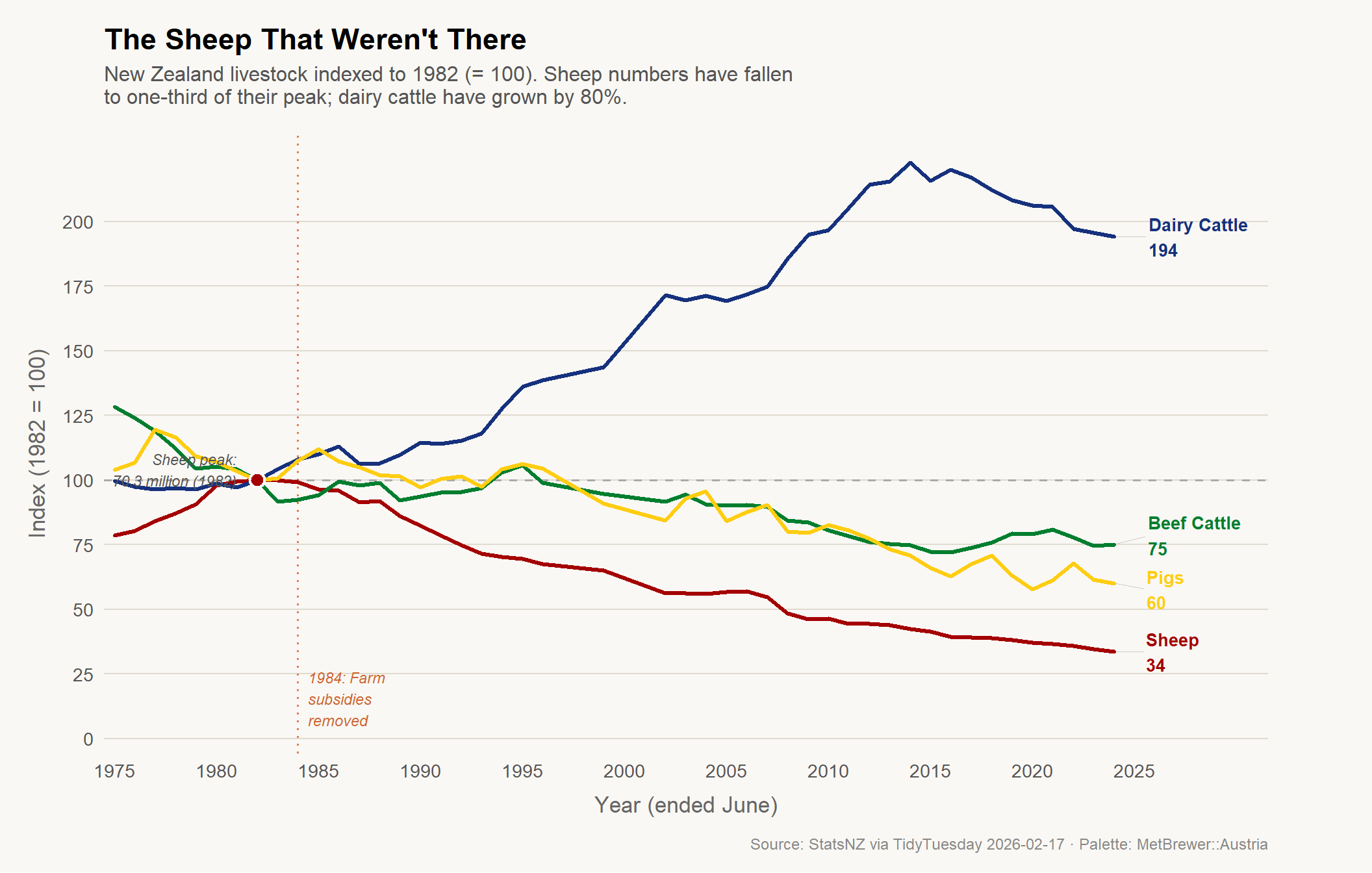
  ggplot2::annotate(
    "text",
    x = 1984.5, y = 5,
    label = "1984: Farm\nsubsidies\nremoved",
    hjust = 0, vjust = 0,
    size = 3, color = "#cc6633", fontface = "italic"
  ) +
  # Annotation: sheep peak
  ggplot2::annotate(
    "point",
    x = 1982, y = 100,
    shape = 21, size = 3.5, fill = pal[1], color = "white", stroke = 1.2
  ) +
  ggplot2::annotate(
    "text",
    x = 1981, y = 104,
    label = "Sheep peak:\n70.3 million (1982)",
    hjust = 1, size = 3, color = "#555555", fontface = "italic"
  ) +
  paletteer::scale_color_paletteer_d("MetBrewer::Austria") +
  ggplot2::scale_x_continuous(
    breaks = seq(1975, 2025, by = 5),
    expand = ggplot2::expansion(mult = c(0.01, 0.12))
  ) +
  ggplot2::scale_y_continuous(
    labels = function(x) paste0(x),
    breaks = seq(0, 200, by = 25)
  ) +
  ggplot2::labs(
    title    = "The Sheep That Weren't There",
    subtitle = "New Zealand livestock indexed to 1982 (= 100). Sheep numbers have fallen\nto one-third of their peak; dairy cattle have grown by 80%.",
    x        = "Year (ended June)",
    y        = "Index (1982 = 100)",
    caption  = "Source: StatsNZ via TidyTuesday 2026-02-17 · Palette: MetBrewer::Austria"
  ) +
  theme_tt

p

Final thoughts and takeaways

New Zealand’s agricultural story is one of the starkest structural economic transitions you can find in a single long-running dataset. Sheep hit 70 million in 1982, a number so outsized it defined the national identity — every New Zealander had roughly 22 sheep looking over their shoulder. Within two decades, the flock had been cut nearly in half.

The 1984 economic reforms were the turning point, not just because subsidies were removed, but because those reforms changed what farming meant in New Zealand. Wool, long the main product, was losing its global market to synthetic fibres. Lamb prices were volatile. Dairy — particularly fresh milk exported to Asia’s growing middle class — offered far better returns per hectare and far more stable contracts. Farmers followed the money, and the pastures followed the farmers.

What the indexed chart reveals that raw numbers obscure: beef cattle have held remarkably steady near their 1982 baseline, confirming that the decline is specific to sheep, not to pastoral farming as a whole. Dairy cattle, meanwhile, grew by roughly 80% above their 1982 level before plateauing and beginning their own modest decline after 2014 — a peak that likely reflects global dairy price cycles and growing environmental pressure on intensive farming near waterways.

The “era of the sheep” spanned roughly 1940–1990. What replaced it was a more complex, more volatile, and in many ways more globally integrated agricultural economy. Whether that’s better for New Zealand’s landscapes, waterways, and rural communities is a separate question the data can only hint at — but the direction of the arrow is unmistakable.

TipFor further reading

New Zealand’s agricultural liberalisation in 1984–1987 remains one of the fastest and most complete removals of farm subsidies in any developed country. The long-run productivity effects are debated, but the livestock data here captures the structural adjustment in real time.