Tidy Tuesday: Golem Grad Tortoise Data

tidytuesday

ecology

herpetology

wildlife

Long-term monitoring of Hermann’s tortoises in the western Balkans reveals a near-perfect relationship between body size and clutch size—and that females consistently outweigh their own shells.

Author

Sean Thimons

Published

March 3, 2026

Preface

From the TidyTuesday repository.

This week’s dataset comes from a long-term mark-recapture study of Hermann’s tortoises (Testudo hermanni) monitored across three localities in the western Balkans. Two datasets are included: body condition index (BCI) measurements collected annually from 2008–2023, and clutch size records paired with morphometric measurements from nesting females. The BCI captures how an individual’s actual body mass compares to the expected mass given its shell length — a proxy for nutritional condition and fat reserves.

Loading necessary packages

My handy booster pack that allows me to install (if needed) and load my usual and favorite packages, as well as some helpful functions.

Code

# Packages ----------------------------------------------------------------

{
  # Install pak if it's not already installed
  if (!requireNamespace("pak", quietly = TRUE)) {
    install.packages(
      "pak",
      repos = sprintf(
        "https://r-lib.github.io/p/pak/stable/%s/%s/%s",
        .Platform$pkgType,
        R.Version()$os,
        R.Version()$arch
      )
    )
  }

  # CRAN Packages ----
  install_booster_pack <- function(package, load = TRUE) {
    for (pkg in package) {
      if (!requireNamespace(pkg, quietly = TRUE)) {
        pak::pkg_install(pkg)
      }
      if (load) {
        library(pkg, character.only = TRUE)
      }
    }
  }

  booster_pack <- c(
    ### IO ----
    'fs',
    'here',
    'janitor',
    'rio',
    'tidyverse',

    ### EDA ----
    'skimr',

    ### Plot ----
    'paletteer',           # Color palette collection
    'patchwork',           # Multi-panel layouts
    'ggrepel',             # Non-overlapping labels
    'ggridges',            # Ridge / joy plots

    ### Misc ----
    'tidytuesdayR'
  )

  install_booster_pack(package = booster_pack, load = TRUE)
  rm(install_booster_pack, booster_pack)

  # Custom Functions ----

  `%ni%` <- Negate(`%in%`)

  geometric_mean <- function(x) {
    exp(mean(log(x[x > 0]), na.rm = TRUE))
  }

  my_skim <- skim_with(
    numeric = sfl(
      n = length,
      min = ~ min(.x, na.rm = T),
      p25 = ~ stats::quantile(., probs = .25, na.rm = TRUE, names = FALSE),
      med = ~ median(.x, na.rm = T),
      p75 = ~ stats::quantile(., probs = .75, na.rm = TRUE, names = FALSE),
      max = ~ max(.x, na.rm = T),
      mean = ~ mean(.x, na.rm = T),
      geo_mean = ~ geometric_mean(.x),
      sd = ~ stats::sd(., na.rm = TRUE),
      hist = ~ inline_hist(., 5)
    ),
    append = FALSE
  )
}

Load raw data from package

raw <- tidytuesdayR::tt_load('2026-03-03')

# Clutch size: nesting females with egg counts and morphometrics
clutch <- raw$clutch_size_cleaned

# Body condition index: repeated annual measurements, 2008–2023
body   <- raw$tortoise_body_condition_cleaned

Exploratory Data Analysis

The my_skim() function is a modified version of skimr::skim() that returns the number of missing data points as well as the inverse, the count, minimum, 25%, median, 75%, max, mean, geometric mean, and standard deviation. It also generates a little ASCII histogram.

Clutch size data

# Drop: individual ID and date (not analytically useful for profiling)
clutch %>%
  select(-individual, -date) %>%
  my_skim()

Data summary
Name	Piped data
Number of rows	53
Number of columns	5
_______________________
Column type frequency:
character	1
numeric	4
________________________
Group variables	None

Variable type: character

skim_variable	n_missing	complete_rate	min	max	empty	n_unique	whitespace
locality	0	1	5	7	0	3	0

Variable type: numeric

skim_variable	complete_rate	n	min	p25	med	p75	max	mean	geo_mean	sd	hist
age	1	53	15	20	22	30	30	24.09	23.53	5.19	▃▅▅▁▇
eggs	1	53	1	3	5	6	11	4.79	4.31	2.11	▇▇▇▁▁
body_mass_grams	1	53	541	1116	1494	1712	2920	1505.04	1404.26	564.60	▆▆▇▃▂
straight_carapace_length_mm	1	53	142	176	192	206	260	191.15	189.25	27.33	▅▅▇▂▂

The clutch dataset is small — 53 observations from nesting females across three localities (Beach, Konjsko, Plateau), ages 15–30 years. Egg counts range from 1 to 11, with a median of 5. Body mass spans from 541 g to nearly 3 kg, and carapace length from 142 mm to 260 mm. The wide ranges across both size measures hint at strong individual variation — and possibly a tight relationship between size and clutch size.

cat("Localities:\n")

Localities:

print(count(clutch, locality))

# A tibble: 3 × 2
  locality     n
  <chr>    <int>
1 Beach       13
2 Konjsko     31
3 Plateau      9

cat("\nAge distribution:\n")


Age distribution:

print(count(clutch, age))

# A tibble: 11 × 2
     age     n
   <dbl> <int>
 1    15     1
 2    16     2
 3    17     3
 4    18     2
 5    19     2
 6    20     6
 7    21     5
 8    22     6
 9    23     2
10    24     3
11    30    21

Body condition data

# Drop: year_recode (redundant with year)
body %>%
  select(-year_recode) %>%
  my_skim()

Data summary
Name	Piped data
Number of rows	10174
Number of columns	8
_______________________
Column type frequency:
character	4
numeric	4
________________________
Group variables	None

Variable type: character

skim_variable	complete_rate	min	max	n_unique
individual	1	1	6	2139
season	1	6	6	2
locality	1	5	7	3
sex	1	1	1	2

Variable type: numeric

skim_variable	complete_rate	n	min	p25	med	p75	max	mean	geo_mean	sd	hist
year	1	10174	2008.00	2011.00	2016.00	2018.00	2023.0	2014.90	2014.90	4.51	▇▂▆▃▃
body_mass_grams	1	10174	528.00	962.00	1092.00	1248.00	2913.0	1133.48	1106.36	263.52	▅▇▁▁▁
body_condition_index	1	10174	3.52	5.66	6.19	6.78	11.7	6.31	6.24	0.98	▁▇▂▁▁
straight_carapace_length_mm	1	10174	150.00	169.00	177.00	185.00	250.0	177.77	177.27	13.36	▅▇▂▁▁

The longitudinal body condition dataset contains 10,174 measurements across 16 years (2008–2023). No missing values. The BCI ranges from 3.5 to ~11.7, centered around 6.1–6.3. The split between Spring and Summer observations is roughly 55/45. Sex coding is "f" and "m" — important to note for filtering later.

cat("Sex values:\n")

Sex values:

print(count(body, sex))

# A tibble: 2 × 2
  sex       n
  <chr> <int>
1 f      1435
2 m      8739

cat("\nLocalities:\n")


Localities:

print(count(body, locality))

# A tibble: 3 × 2
  locality     n
  <chr>    <int>
1 Beach      618
2 Konjsko   1616
3 Plateau   7940

cat("\nSeasons:\n")


Seasons:

print(count(body, season))

# A tibble: 2 × 2
  season     n
  <chr>  <int>
1 Spring  5747
2 Summer  4427

cat("\nBCI by sex (mean ± SD):\n")


BCI by sex (mean ± SD):

body %>%
  group_by(sex) %>%
  summarize(
    n        = n(),
    mean_bci = round(mean(body_condition_index), 3),
    sd_bci   = round(sd(body_condition_index), 3),
    .groups  = "drop"
  ) %>%
  print()

# A tibble: 2 × 4
  sex       n mean_bci sd_bci
  <chr> <int>    <dbl>  <dbl>
1 f      1435     7.48  1.37 
2 m      8739     6.12  0.742

cat("\nBCI by locality:\n")


BCI by locality:

body %>%
  group_by(locality) %>%
  summarize(
    n        = n(),
    mean_bci = round(mean(body_condition_index), 3),
    .groups  = "drop"
  ) %>%
  print()

# A tibble: 3 × 3
  locality     n mean_bci
  <chr>    <int>    <dbl>
1 Beach      618     5.80
2 Konjsko   1616     7.46
3 Plateau   7940     6.12

The EDA reveals two striking patterns:

Sex gap: Females average BCI 7.48 vs. males 6.12 — more than a full unit difference, with females showing substantially wider spread (SD 1.37 vs. 0.74).
Locality gap: Konjsko individuals score highest (BCI 7.46), well above Beach (5.80) and Plateau (6.12).

These patterns motivate the two analytical threads below.

Body condition: who’s in the best shape, and where?

The body condition index here is a residual measure — it captures how much an individual’s actual body mass deviates from the expected mass given its shell length. Higher BCI means the animal is carrying more mass relative to its structural size, a proxy for fat reserves and nutritional status.

Note

In reptiles, elevated fat reserves in females are not simply a sign of good health — they’re a reproductive necessity. Female tortoises must accumulate substantial lipid stores prior to egg formation. The ~22% BCI advantage females show over males in this dataset is likely a direct reflection of that investment.

# Verify sex × locality combination counts before plotting
bci_plot_data <- body %>%
  mutate(
    sex_label = ifelse(sex == "f", "Female", "Male"),
    sex_label = factor(sex_label, levels = c("Female", "Male"))
  )

cat(sprintf("bci_plot_data: %d rows, %d cols\n", nrow(bci_plot_data), ncol(bci_plot_data)))

bci_plot_data: 10174 rows, 10 cols

stopifnot("Plot data has 0 rows" = nrow(bci_plot_data) > 0)

# Check actual BCI range is sensible
bci_range <- range(bci_plot_data$body_condition_index)
cat(sprintf("BCI range: %.2f – %.2f\n", bci_range[1], bci_range[2]))

BCI range: 3.52 – 11.70

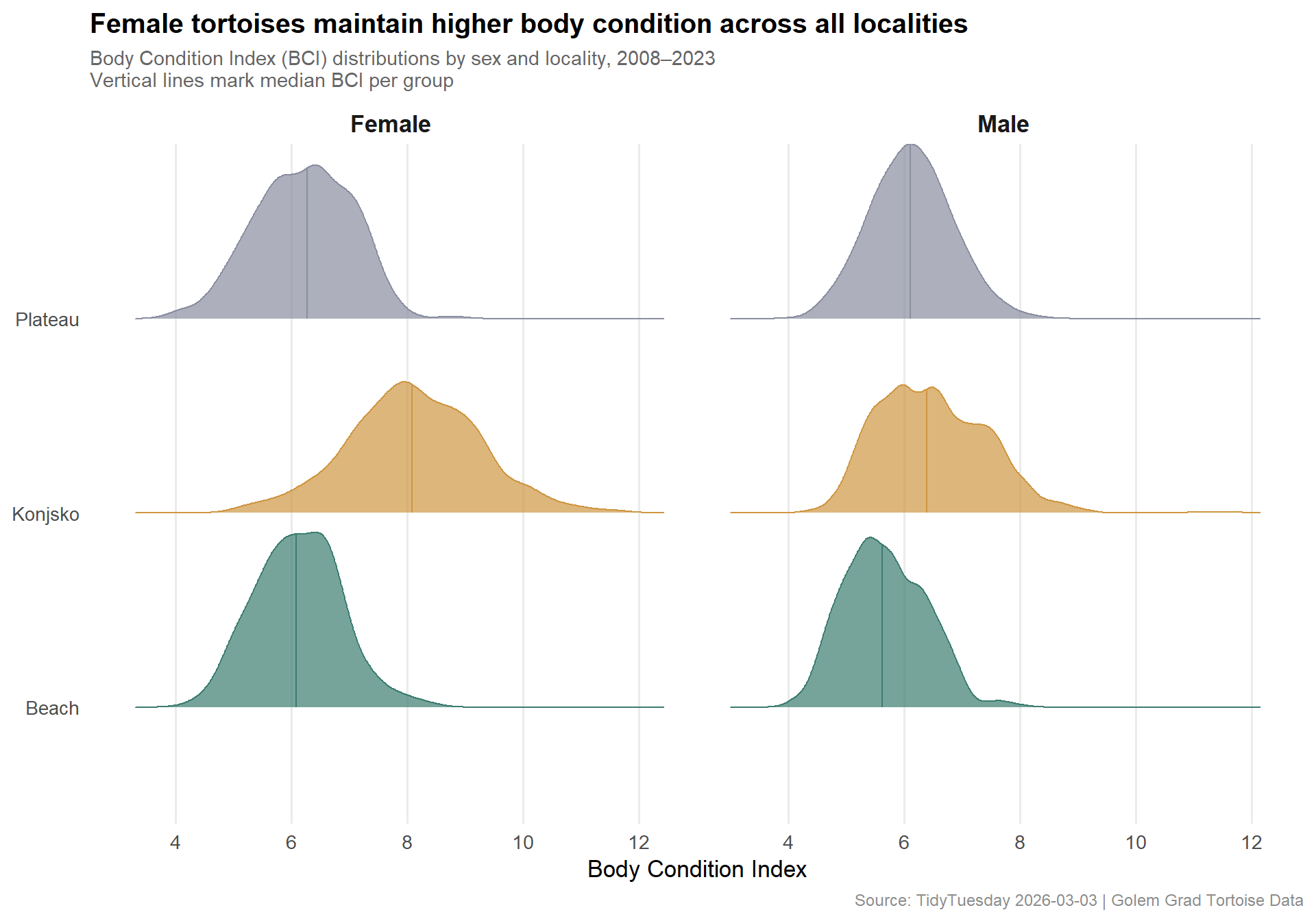
locality_colors <- paletteer::paletteer_d("MetBrewer::Kandinsky", n = 3)
names(locality_colors) <- c("Beach", "Konjsko", "Plateau")

p_bci <- ggplot2::ggplot(
  bci_plot_data,
  ggplot2::aes(
    x    = body_condition_index,
    y    = locality,
    fill = locality,
    color = locality
  )
) +
  ggridges::geom_density_ridges(
    alpha        = 0.7,
    scale        = 0.9,
    quantile_lines = TRUE,
    quantiles    = 2,        # median line
    jittered_points = FALSE
  ) +
  ggplot2::facet_wrap(~sex_label, ncol = 2) +
  ggplot2::scale_fill_manual(values = locality_colors) +
  ggplot2::scale_color_manual(values = locality_colors) +
  ggplot2::scale_x_continuous(breaks = seq(4, 12, by = 2)) +
  ggplot2::labs(
    title    = "Female tortoises maintain higher body condition across all localities",
    subtitle = "Body Condition Index (BCI) distributions by sex and locality, 2008–2023\nVertical lines mark median BCI per group",
    x        = "Body Condition Index",
    y        = NULL,
    fill     = "Locality",
    color    = "Locality",
    caption  = "Source: TidyTuesday 2026-03-03 | Golem Grad Tortoise Data"
  ) +
  ggplot2::theme_minimal(base_size = 13) +
  ggplot2::theme(
    plot.title         = ggplot2::element_text(face = "bold", size = 15),
    plot.subtitle      = ggplot2::element_text(color = "gray40", size = 11),
    plot.caption       = ggplot2::element_text(color = "gray55", size = 9),
    strip.text         = ggplot2::element_text(face = "bold", size = 13),
    legend.position    = "none",
    panel.grid.minor   = ggplot2::element_blank(),
    panel.grid.major.y = ggplot2::element_blank()
  )

p_bci

The ridge distributions tell a clear story. For females, the Konjsko population is shifted markedly rightward — a heavy right tail reaching past BCI 10. Beach and Plateau females overlap considerably but trail Konjsko by a full unit at the median. For males, distributions are tighter and more uniform across localities, all clustering around BCI 5.5–6.5. The male Konjsko advantage disappears in the tight BCI range.

This locality × sex interaction suggests that Konjsko habitat uniquely enables females to achieve the elevated fat deposits necessary for robust egg production — a pattern we can test directly with the clutch data.

Body size predicts reproductive output

# Verify actual locality values in the clutch dataset
cat("Localities in clutch data:\n")

Localities in clutch data:

print(sort(unique(clutch$locality)))

[1] "Beach"   "Konjsko" "Plateau"

# Confirm these match the BCI dataset
stopifnot(all(clutch$locality %in% c("Beach", "Konjsko", "Plateau")))

cat(sprintf("clutch: %d rows, %d cols\n", nrow(clutch), ncol(clutch)))

clutch: 53 rows, 7 cols

stopifnot("clutch has 0 rows" = nrow(clutch) > 0)

# Correlation statistics
cor_mass  <- cor.test(clutch$body_mass_grams, clutch$eggs)
cor_scl   <- cor.test(clutch$straight_carapace_length_mm, clutch$eggs)

cat(sprintf("\nBody mass × eggs:    r = %.3f, p < 2.2e-16\n", cor_mass$estimate))


Body mass × eggs:    r = 0.896, p < 2.2e-16

cat(sprintf("Carapace × eggs:     r = %.3f, p < 2.2e-16\n", cor_scl$estimate))

Carapace × eggs:     r = 0.882, p < 2.2e-16

# Sanity check: are eggs proportional values or counts?
cat(sprintf("\nEgg count range: %d – %d (should be counts, not proportions)\n",
            min(clutch$eggs), max(clutch$eggs)))


Egg count range: 1 – 11 (should be counts, not proportions)

if (max(clutch$eggs) <= 1) {
  warning("Eggs column looks like proportions, not counts — check data")
}

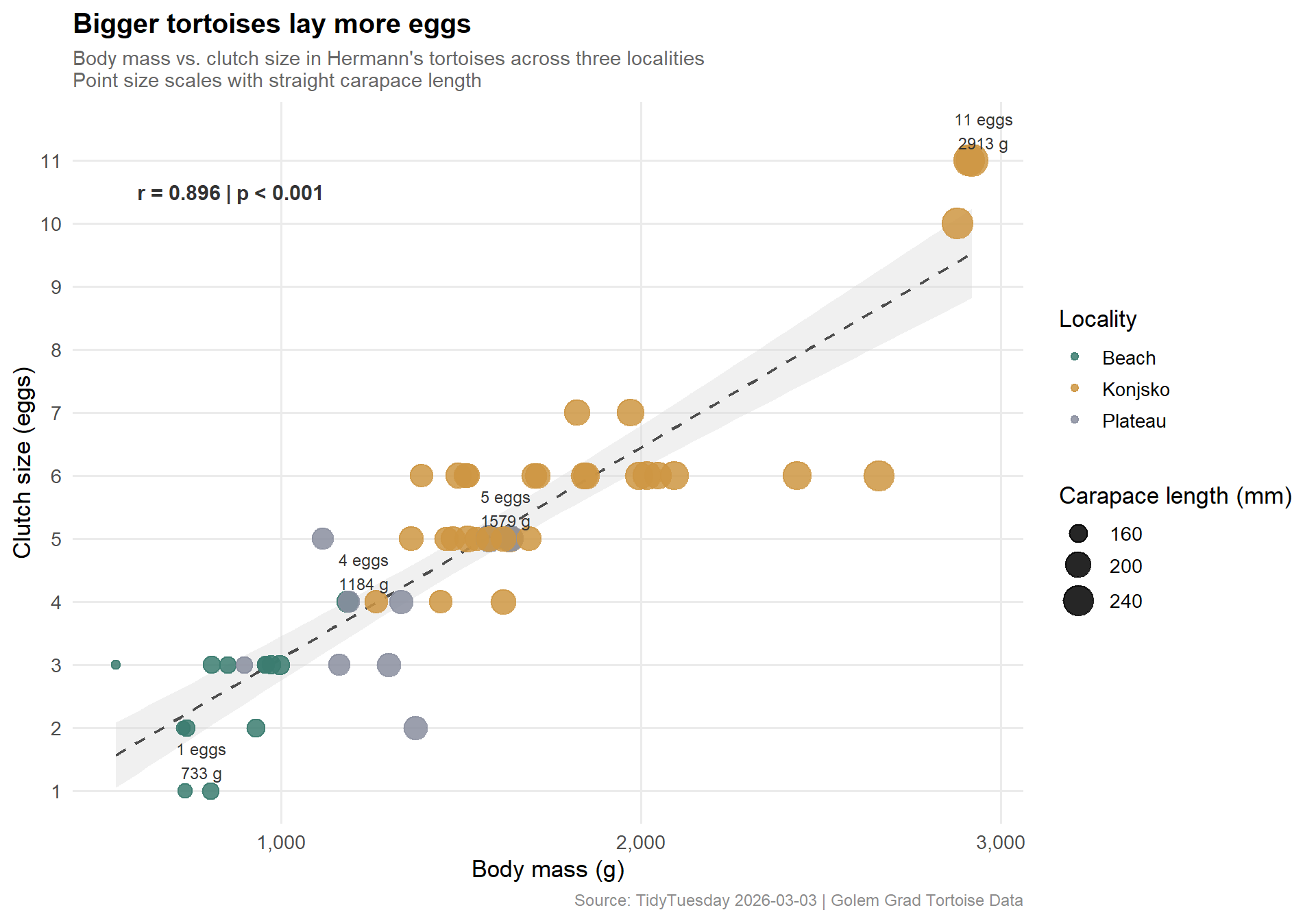
The Pearson correlation between body mass and clutch size is r = 0.896 (p < 2.2e–16). For a biological dataset with only 53 observations spanning wild-caught individuals across multiple years, this is a remarkably tight relationship. Carapace length shows nearly identical predictive power (r = 0.882).

Important

What r = 0.896 means in practice: roughly 80% of the variance in egg count is accounted for by body mass alone. The largest female in the sample (2,920 g) laid 11 eggs; the smallest (541 g) laid 1. That’s an 11-fold range in reproductive output explained almost entirely by how big the animal is.

# Label outliers: largest clutch per locality, and the minimum
label_pts <- bind_rows(
  clutch %>%
    group_by(locality) %>%
    slice_max(order_by = eggs, n = 1, with_ties = FALSE),
  clutch %>%
    slice_min(order_by = eggs, n = 1, with_ties = FALSE)
) %>%
  distinct(individual, .keep_all = TRUE) %>%
  mutate(label = paste0(eggs, " eggs\n", body_mass_grams, " g"))

cat(sprintf("label_pts: %d rows\n", nrow(label_pts)))

label_pts: 4 rows

p_scatter <- ggplot2::ggplot(
  clutch,
  ggplot2::aes(x = body_mass_grams, y = eggs, color = locality)
) +
  ggplot2::geom_smooth(
    method    = "lm",
    se        = TRUE,
    color     = "gray30",
    fill      = "gray85",
    linewidth = 0.8,
    linetype  = "dashed"
  ) +
  ggplot2::geom_point(
    ggplot2::aes(size = straight_carapace_length_mm),
    alpha = 0.85
  ) +
  ggrepel::geom_text_repel(
    data        = label_pts,
    ggplot2::aes(label = label),
    size        = 3.2,
    nudge_y     = 0.4,
    nudge_x     = 30,
    color       = "gray20",
    segment.color = "gray60",
    segment.size  = 0.4,
    box.padding   = 0.4
  ) +
  ggplot2::scale_color_manual(values = locality_colors) +
  ggplot2::scale_size_continuous(
    name   = "Carapace length (mm)",
    range  = c(2, 8),
    breaks = c(160, 200, 240)
  ) +
  ggplot2::annotate(
    "text",
    x     = 600,
    y     = 10.5,
    label = "r = 0.896 | p < 0.001",
    hjust = 0,
    size  = 4,
    color = "gray20",
    fontface = "bold"
  ) +
  ggplot2::scale_x_continuous(labels = scales::comma) +
  ggplot2::scale_y_continuous(breaks = 1:11) +
  ggplot2::labs(
    title    = "Bigger tortoises lay more eggs",
    subtitle = "Body mass vs. clutch size in Hermann's tortoises across three localities\nPoint size scales with straight carapace length",
    x        = "Body mass (g)",
    y        = "Clutch size (eggs)",
    color    = "Locality",
    caption  = "Source: TidyTuesday 2026-03-03 | Golem Grad Tortoise Data"
  ) +
  ggplot2::theme_minimal(base_size = 13) +
  ggplot2::theme(
    plot.title       = ggplot2::element_text(face = "bold", size = 15),
    plot.subtitle    = ggplot2::element_text(color = "gray40", size = 11),
    plot.caption     = ggplot2::element_text(color = "gray55", size = 9),
    panel.grid.minor = ggplot2::element_blank(),
    legend.position  = "right"
  )

p_scatter

The scatter makes the relationship almost uncomfortable in its linearity — these points want to fall on a line. Konjsko individuals (amber) tend to cluster in the upper-right corner (high mass, high clutch size), consistent with the BCI advantage we saw in the ridge plots. Beach tortoises (teal) appear mostly at mid-mass; the single Plateau point near the top right is a notable outlier.

Log palette

Final thoughts and takeaways

This dataset from a Balkan Hermann’s tortoise study turns out to be a compact illustration of two intertwined ecological principles:

Body condition is sex-stratified by design. The ~22% BCI gap between females and males isn’t a sign that males are unhealthy — it reflects the asymmetric energetic demands of reproduction. Females must mobilize fat reserves to produce calcified eggs; males don’t. Konjsko amplifies this effect, suggesting better vegetation cover or food availability that enables females there to achieve the highest pre-nesting condition in the dataset. This locality-level effect has real conservation implications: habitat degradation at Konjsko would disproportionately harm female reproductive success.

Size is reproductive destiny, at r = 0.896. This correlation is extremely high for a wild biological dataset. It means that a female tortoise’s body mass is, in practice, a near-sufficient predictor of how many eggs she will lay — more than age, year, or locality alone. Since tortoises grow slowly and live for decades, this finding elevates early life conditions (juvenile growth rates, food availability) as critical determinants of lifetime reproductive output. A tortoise that grows slowly in its first decade carries that reproductive penalty for life.

Limitations: The clutch size dataset is small (n = 53) and restricted to females who were observed nesting — likely biased toward better-condition individuals who successfully nested. The BCI data is far richer but tracks a narrow three-locality window of a much wider species range. Generalizing these patterns to other T. hermanni populations requires caution.

The overall picture, though, is coherent: take care of the habitat, the females grow bigger, and they lay more eggs. That’s a tractable conservation lever.