Tidy Tuesday: Coastal Ocean Temperature by Depth

Exploring vertical temperature profiles in Lunenburg County’s coastal waters.

Preface

From TidyTuesday repository.

This dataset explores the complex relationship between ocean depth and mean water temperature in coastal monitoring sites.

Loading necessary packages

My handy booster pack that allows me to install (if needed) and load my usual and favorite packages, as well as some helpful functions.

# Packages ----------------------------------------------------------------

{
  # Install pak if it's not already installed
  if (!requireNamespace("pak", quietly = TRUE)) {
    install.packages("pak", repos = "https://cloud.r-project.org")
  }

  # CRAN Packages ----
  install_booster_pack <- function(package, load = TRUE) {
    for (pkg in package) {
      if (!requireNamespace(pkg, quietly = TRUE)) {
        pak::pkg_install(pkg)
      }
      if (load) {
        library(pkg, character.only = TRUE)
      }
    }
  }

  core_packages <- c(
    'fs',
    'here',
    'janitor',
    'rio',
    'tidyverse',
    'skimr',
    'paletteer',
    'tidytuesdayR'
  )

  optional_packages <- c('gghighlight', 'ggthemes', 'patchwork')

  install_booster_pack(package = unique(c(core_packages, optional_packages)), load = TRUE)
  rm(install_booster_pack, core_packages, optional_packages)

  # Custom Functions ----

  `%ni%` <- Negate(`%in%`)

  geometric_mean <- function(x) {
    exp(mean(log(x[x > 0]), na.rm = TRUE))
  }

  my_skim <- skim_with(
    numeric = sfl(
      n = length,
      min = ~ min(.x, na.rm = T),
      p25 = ~ stats::quantile(., probs = .25, na.rm = TRUE, names = FALSE),
      med = ~ median(.x, na.rm = T),
      p75 = ~ stats::quantile(., probs = .75, na.rm = TRUE, names = FALSE),
      max = ~ max(.x, na.rm = T),
      mean = ~ mean(.x, na.rm = T),
      geo_mean = ~ geometric_mean(.x),
      sd = ~ stats::sd(., na.rm = TRUE),
      hist = ~ inline_hist(., 5)
    ),
    append = FALSE
  )
}

Load raw data from package

raw <- tidytuesdayR::tt_load('2026-03-31')

ocean_temp <- raw$ocean_temperature
deployments <- raw$ocean_temperature_deployments

Exploratory Data Analysis

The my_skim() function is a modified version of the skimr::skim() function that returns the number of missing data points (cells as NA) as well as the inverse (e.g.: number of rows that are not NA), the count, minimum, 25%, median, 75%, max, mean, geometric mean, and standard deviation. It also generates a little ASCII histogram. Neat!

Ocean Temperature Data

my_skim(ocean_temp)

Data summary

Name	ocean_temp
Number of rows	19165
Number of columns	5
_______________________
Column type frequency:
Date	1
numeric	4
________________________
Group variables	None

Variable type: Date

skim_variable	n_missing	complete_rate	min	max	median	n_unique
date	0	1	2018-02-20	2025-12-06	2021-12-10	2847

Variable type: numeric

skim_variable	n_missing	complete_rate	n	min	p25	med	p75	max	mean	geo_mean	sd	hist
sensor_depth_at_low_tide_m	0	1	19165	2.00	5.00	15.00	30.00	40.00	17.57	12.34	12.48	▇▇▃▃▃
mean_temperature_degree_c	0	1	19165	0.31	3.33	5.65	9.34	21.32	6.95	5.51	4.65	▇▇▃▂▁
sd_temperature_degree_c	0	1	19165	0.00	0.08	0.16	0.35	4.71	0.30	0.17	0.40	▇▁▁▁▁
n_obs	0	1	19165	8.00	96.00	96.00	96.00	1440.00	99.42	89.79	60.17	▇▁▁▁▁

The dataset contains vertical temperature measurements across multiple depths. We see a clear depth-temperature gradient.

Seasonal Stability vs Depth

How does the variance (standard deviation) of temperature behave as we go deeper? We might expect deeper waters to be more thermally stable throughout the year.

p <- ocean_temp %>%
  mutate(month = month(date, label = TRUE)) %>%
  group_by(sensor_depth_at_low_tide_m, month) %>%
  summarize(
    mean_temp = mean(mean_temperature_degree_c, na.rm = TRUE),
    sd_temp = mean(sd_temperature_degree_c, na.rm = TRUE),
    .groups = "drop"
  ) %>%
  ggplot(aes(x = month, y = mean_temp, group = factor(sensor_depth_at_low_tide_m))) +
  geom_line(aes(color = sensor_depth_at_low_tide_m), linewidth = 1.2) +
  scale_color_paletteer_c("scico::oslo", direction = -1) +
  labs(
    title = "Mean Ocean Temperature Cycles by Sensor Depth",
    subtitle = "Deepest sensors (darker) show more stability and slightly warmer winter mins",
    x = "Month",
    y = "Mean Temperature (°C)",
    color = "Depth (m)"
  ) +
  theme_minimal() +
  theme(
    legend.position = "bottom",
    plot.title = element_text(face = "bold"),
    panel.grid.minor = element_blank()
  )

p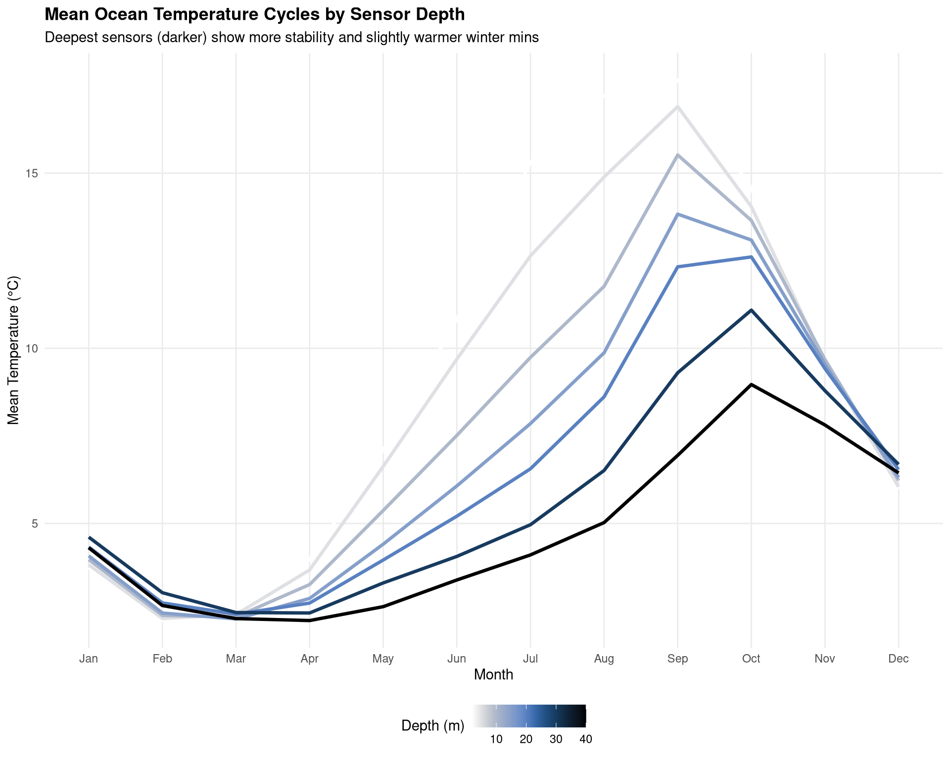

Final thoughts and takeaways

The data confirms that while the surface waters experience the most extreme swings, the deeper strata provide a more stable thermal environment, which is critical for local sea life during the transition seasons.