
Tidy Tuesday: Bird Sightings at Sea
tidytuesday
R
birds
ecology
ocean
Which Southern Ocean seabirds chase ships, and which ones just fly on by? A look at three decades of pelagic bird observations from research vessels in the Australasian seas.
Preface
From TidyTuesday repository.
Between 1969 and 1990, naturalists aboard New Zealand and Australian research vessels recorded every seabird they could spot from the deck, along with the ship’s position, weather, sea state, and what the birds were doing. The result is a remarkable archive of pelagic seabird behavior in the Southern Ocean — albatrosses, petrels, shearwaters, and gulls — across more than 12,000 ship records and 49,000 individual sightings. Each row tells you not just what was seen, but whether it was following the ship, sitting on the water, flying past, or feeding.
The four tables in this week’s release split the work neatly: ships carries the position/time/weather context, birds carries the sightings keyed back to each ship record, and the two small lookup tables encode the Beaufort wind scale and World Meteorological Organization sea-state class.
Loading necessary packages
My handy booster pack that allows me to install (if needed) and load my usual and favorite packages, as well as some helpful functions.
Code
{
  if (!requireNamespace("pak", quietly = TRUE)) {
    install.packages("pak", repos = "https://cloud.r-project.org")
  }

  install_booster_pack <- function(package, load = TRUE) {
    for (pkg in package) {
      if (!requireNamespace(pkg, quietly = TRUE)) {
        pak::pkg_install(pkg)
      }
      if (load) {
        library(pkg, character.only = TRUE)
      }
    }
  }

  core_packages <- c(
    'fs',
    'here',
    'janitor',
    'rio',
    'tidyverse',
    'skimr',
    'paletteer',
    'tidytuesdayR'
  )

  optional_packages <- c('ggtext', 'ggrepel', 'scales', 'lubridate')

  install_booster_pack(package = unique(c(core_packages, optional_packages)), load = TRUE)
  rm(install_booster_pack, core_packages, optional_packages)

  `%ni%` <- Negate(`%in%`)

  geometric_mean <- function(x) {
    exp(mean(log(x[x > 0]), na.rm = TRUE))
  }

  my_skim <- skim_with(
    numeric = sfl(
      n = length,
      min = ~ min(.x, na.rm = T),
      p25 = ~ stats::quantile(., probs = .25, na.rm = TRUE, names = FALSE),
      med = ~ median(.x, na.rm = T),
      p75 = ~ stats::quantile(., probs = .75, na.rm = TRUE, names = FALSE),
      max = ~ max(.x, na.rm = T),
      mean = ~ mean(.x, na.rm = T),
      geo_mean = ~ geometric_mean(.x),
      sd = ~ stats::sd(., na.rm = TRUE),
      hist = ~ inline_hist(., 5)
    ),
    append = FALSE
  )
}
Load raw data from package
raw <- tidytuesdayR::tt_load('2026-04-14')

ships          <- raw$ships
birds          <- raw$birds
beaufort_scale <- raw$beaufort_scale
sea_states     <- raw$sea_states
Exploratory Data Analysis
The my_skim() function is a modified version of skimr::skim() that returns the number of missing data points (cells as NA) as well as the inverse (e.g.: number of rows that are not NA), the count, minimum, 25%, median, 75%, max, mean, geometric mean, and standard deviation. It also generates a little ASCII histogram. Neat!
Ships
ships %>%
  select(-record_id, -observer) %>%
my_skim()| Name | Piped data |
| Number of rows | 12310 |
| Number of columns | 19 |
| _______________________ | |
| Column type frequency: | |
| character | 6 |
| Date | 1 |
| difftime | 1 |
| numeric | 11 |
| ________________________ | |
| Group variables | None |
Variable type: character
| skim_variable | n_missing | complete_rate | min | max | empty | n_unique | whitespace |
|---|---|---|---|---|---|---|---|
| hemisphere | 11 | 1.00 | 1 | 1 | 0 | 2 | 0 |
| activity | 0 | 1.00 | 7 | 18 | 0 | 7 | 0 |
| cloud_cover | 4787 | 0.61 | 5 | 16 | 0 | 3 | 0 |
| precipitation | 4803 | 0.61 | 3 | 15 | 0 | 8 | 0 |
| census_method | 0 | 1.00 | 4 | 7 | 0 | 2 | 0 |
| season | 0 | 1.00 | 6 | 6 | 0 | 4 | 0 |
Variable type: Date
| skim_variable | n_missing | complete_rate | min | max | median | n_unique |
|---|---|---|---|---|---|---|
| date | 0 | 1 | 1969-07-31 | 1990-12-21 | 1984-02-17 | 1435 |
Variable type: difftime
| skim_variable | n_missing | complete_rate | min | max | median | n_unique |
|---|---|---|---|---|---|---|
| time | 2 | 1 | 0 secs | 84600 secs | 45600 secs | 315 |
Variable type: numeric
| skim_variable | n_missing | complete_rate | n | min | p25 | med | p75 | max | mean | geo_mean | sd | hist |
|---|---|---|---|---|---|---|---|---|---|---|---|---|
| latitude | 10 | 1.00 | 12310 | -69.0 | -40.6 | -38.27 | -35.50 | -19.00 | -39.22 | NaN | 5.89 | ▁▁▆▇▁ |
| longitude | 11 | 1.00 | 12310 | 50.0 | 152.0 | 163.12 | 172.92 | 179.98 | 159.93 | 158.72 | 17.42 | ▁▁▁▃▇ |
| speed | 4478 | 0.64 | 12310 | 0.0 | 10.5 | 14.50 | 16.00 | 22.00 | 12.71 | 13.12 | 5.18 | ▂▁▅▇▂ |
| direction | 11055 | 0.10 | 12310 | 0.0 | 90.0 | 165.00 | 270.00 | 358.00 | 169.35 | 128.89 | 102.47 | ▅▇▅▅▅ |
| wind_speed_class | 4688 | 0.62 | 12310 | 0.0 | 2.0 | 4.00 | 5.00 | 12.00 | 3.73 | 3.40 | 1.83 | ▅▇▆▁▁ |
| wind_direction | 11018 | 0.10 | 12310 | 0.0 | 68.0 | 203.00 | 270.00 | 350.00 | 174.71 | 157.63 | 108.50 | ▇▃▃▇▆ |
| air_temperature | 11274 | 0.08 | 12310 | 0.5 | 13.4 | 15.50 | 17.80 | 24.60 | 15.28 | 14.52 | 3.83 | ▁▁▅▇▂ |
| pressure | 11540 | 0.06 | 12310 | 991.0 | 1010.0 | 1016.00 | 1021.00 | 1040.00 | 1014.84 | 1014.80 | 8.85 | ▁▃▇▅▁ |
| sea_state_class | 4751 | 0.61 | 12310 | 1.0 | 3.0 | 4.00 | 4.00 | 6.00 | 3.56 | 3.33 | 1.10 | ▂▇▆▃▁ |
| sea_surface_temperature | 11625 | 0.06 | 12310 | -1.0 | 12.8 | 15.10 | 17.00 | 27.00 | 14.72 | 14.08 | 4.08 | ▁▁▇▆▁ |
| depth | 12180 | 0.01 | 12310 | 60.0 | 162.5 | 290.00 | 507.50 | 2200.00 | 380.85 | 283.99 | 352.05 | ▇▂▁▁▁ |
ships %>%
  count(season, name = "n_ship_records") %>%
  arrange(desc(n_ship_records))
# A tibble: 4 × 2
season n_ship_records
<chr> <int>
1 spring 3585
2 summer 3477
3 autumn 2794
4 winter 2454ships %>%
summarise(
first_voyage = min(date, na.rm = TRUE),
last_voyage = max(date, na.rm = TRUE),
n_records = n(),
lat_min = min(latitude, na.rm = TRUE),
lat_max = max(latitude, na.rm = TRUE),
lon_min = min(longitude, na.rm = TRUE),
lon_max = max(longitude, na.rm = TRUE)
)# A tibble: 1 × 7
first_voyage last_voyage n_records lat_min lat_max lon_min lon_max
<date> <date> <int> <dbl> <dbl> <dbl> <dbl>
1 1969-07-31 1990-12-21 12310 -69 -19 50 180.The fleet works almost exclusively in the eastern hemisphere (hemisphere == "E"), wedged between roughly 19°S and 69°S — that’s the swath from sub-tropical Tasman waters down through the Roaring Forties, Furious Fifties, and into the Antarctic Convergence. Records span late July 1969 through December 1990 and are evenly spread across all four seasons, with a slight lean toward spring and summer when the southern weather permits more deck time.
Birds
birds %>%
  select(species_common_name, age, plumage_phase, count,
         following_ship, flying_past, sitting_on_water, feeding) %>%
my_skim()| Name | Piped data |
| Number of rows | 49019 |
| Number of columns | 8 |
| _______________________ | |
| Column type frequency: | |
| character | 3 |
| logical | 4 |
| numeric | 1 |
| ________________________ | |
| Group variables | None |
Variable type: character
| skim_variable | n_missing | complete_rate | min | max | empty | n_unique | whitespace |
|---|---|---|---|---|---|---|---|
| species_common_name | 691 | 0.99 | 9 | 56 | 0 | 321 | 0 |
| age | 38837 | 0.21 | 5 | 8 | 0 | 4 | 0 |
| plumage_phase | 48938 | 0.00 | 4 | 12 | 0 | 4 | 0 |
Variable type: logical
| skim_variable | n_missing | complete_rate | mean | count |
|---|---|---|---|---|
| following_ship | 21132 | 0.57 | 0.42 | FAL: 16068, TRU: 11819 |
| flying_past | 21128 | 0.57 | 0.42 | FAL: 16163, TRU: 11728 |
| sitting_on_water | 21122 | 0.57 | 0.12 | FAL: 24427, TRU: 3470 |
| feeding | 21095 | 0.57 | 0.13 | FAL: 24320, TRU: 3604 |
Variable type: numeric
| skim_variable | n_missing | complete_rate | n | min | p25 | med | p75 | max | mean | geo_mean | sd | hist |
|---|---|---|---|---|---|---|---|---|---|---|---|---|
| count | 2699 | 0.94 | 49019 | 1 | 1 | 2 | 4 | 99999 | 41.93 | 2.46 | 1283.41 | ▇▁▁▁▁ |
birds %>%
  count(species_common_name, sort = TRUE) %>%
  head(10)
# A tibble: 10 × 2
species_common_name n
<chr> <int>
1 Wandering albatross sensu lato PL2 3104
2 Cape petrel 2936
3 Wandering albatross sensu lato PL3 2885
4 Grey-faced petrel 2597
5 Giant petrel sensu lato 2094
6 Prion (unidentified) 2094
7 Wandering albatross sensu lato PL1 1818
8 Black-browed albatross sensu lato AD 1805
9 Wandering albatross sensu lato PL4 1475
10 Australasian gannet AD 1366birds %>%
summarise(
pct_following = mean(following_ship, na.rm = TRUE),
pct_flying = mean(flying_past, na.rm = TRUE),
pct_sitting = mean(sitting_on_water, na.rm = TRUE),
pct_feeding = mean(feeding, na.rm = TRUE)
)# A tibble: 1 × 4
pct_following pct_flying pct_sitting pct_feeding
<dbl> <dbl> <dbl> <dbl>
1 0.424 0.420 0.124 0.129The bird table is dominated by tubenoses — albatrosses, petrels, shearwaters, and prions. The single most-sighted “species” is the wandering albatross sensu lato in plumage phase 2, with over 3,000 records. (The “sensu lato” tag and PL1–PL5 codes flag that field observers were grouping look-alike sub-taxa and ageing them by their plumage transition, since wandering albatrosses take roughly a decade to reach definitive adult white.)
Roughly 42% of behaviorally-scored sightings record a bird actively following the ship — an extraordinary fraction, but consistent with what mariners have reported since the age of sail: certain seabirds, especially albatrosses, treat a vessel as a slow-moving feeding opportunity (offal, prop wash, disturbed plankton). The behavior is not uniform, though — and that variation is the story.
Which seabirds follow ships?
The “ship-follower” trade-off
Following a vessel costs energy — sustained flight, sometimes for hours — but pays out in the form of galley scraps, churned-up prey, and easy soaring on the ship’s wake-edge updrafts. Species that evolved to scavenge over vast empty ocean (albatrosses, giant petrels) take that bet readily. Species that pluck prey from the water surface in fast dives or that follow specific schooling fish (shearwaters, gannets) tend to ignore the ship entirely.
I want to rank species by the fraction of individual birds observed actively following the ship — not just the fraction of sightings, because flocks of dozens are common and one record can represent very different numbers of birds. To avoid the noise of rarely-seen species, I’ll restrict to species with at least 250 records on file, and collapse the wandering-albatross plumage codes into a single species group.
bird_ship <- birds %>%
  inner_join(ships, by = "record_id") %>%
  filter(!is.na(species_common_name)) %>%
  mutate(
    species_grp = species_common_name %>%
      str_replace(" sensu lato.*$", "") %>%
      str_replace("\\s+(AD|JUV|SUB.*|PL\\d+).*$", "") %>%
      str_trim()
  )

follow_summary <- bird_ship %>%
  group_by(species_grp) %>%
  summarise(
    n_records          = n(),
    total_birds        = sum(count, na.rm = TRUE),
    birds_following    = sum(n_following_ship, na.rm = TRUE),
    birds_flying_past  = sum(n_flying_past,    na.rm = TRUE),
    birds_sitting      = sum(n_sitting_on_water, na.rm = TRUE),
    birds_feeding      = sum(n_feeding,        na.rm = TRUE),
    .groups = "drop"
  ) %>%
  filter(n_records >= 250, total_birds > 0) %>%
  mutate(
    pct_following = birds_following   / total_birds,
    pct_flying    = birds_flying_past / total_birds,
    pct_sitting   = birds_sitting     / total_birds
  ) %>%
  arrange(desc(pct_following))

cat(sprintf("follow_summary: %d species after filtering\n", nrow(follow_summary)))
follow_summary: 35 species after filteringstopifnot("follow_summary is empty — check joins/filters" = nrow(follow_summary) > 0)
follow_summary %>%
select(species_grp, n_records, total_birds, pct_following, pct_flying, pct_sitting) %>%
print(n = Inf)# A tibble: 35 × 6
species_grp n_records total_birds pct_following pct_flying pct_sitting
<chr> <int> <dbl> <dbl> <dbl> <dbl>
1 White-chinned pet… 489 1246 0.474 0.104 0.0241
2 Wandering albatro… 11293 19905 0.468 0.00769 0.0121
3 Black petrel 403 1799 0.314 0.0506 0.0634
4 Black-browed alba… 3609 9057 0.308 0.0194 0.0153
5 Light-mantled soo… 259 679 0.239 0.0707 0.00295
6 Cape petrel 2936 25790 0.183 0.00578 0.0238
7 Giant petrel 2168 5533 0.169 0.00886 0.0134
8 Wilson's storm pe… 257 654 0.122 0.243 0.00153
9 Pomarine skua 308 980 0.0459 0.140 0.00510
10 Flesh-footed shea… 849 9824 0.0457 0.104 0.0932
11 Yellow-nosed moll… 684 1438 0.0376 0.153 0.146
12 Westland / White-… 371 1334 0.0337 0.114 0.124
13 White-headed petr… 558 1403 0.0321 0.383 0.271
14 Red-billed gull 754 11323 0.0273 0.0185 0.0646
15 Buller's mollymawk 312 778 0.0231 0.239 0.0578
16 Westland petrel 399 2662 0.0214 0.193 0.246
17 Great-winged / Gr… 369 1238 0.0210 0.269 0.0121
18 Southern black-ba… 1413 10281 0.0190 0.00953 0.128
19 Grey-faced petrel 2597 10368 0.0129 0.314 0.0909
20 Black-winged petr… 453 1192 0.00671 0.375 0.0143
21 Shy / White-cappe… 383 2693 0.00668 0.105 0.0319
22 Australasian gann… 1676 27037 0.00544 0.0818 0.0947
23 Shy / white-cappe… 1534 5576 0.00538 0.0959 0.174
24 Gould's petrel 350 775 0.00387 0.488 0.0271
25 Salvin's mollymawk 275 857 0.00350 0.104 0.0968
26 Crested tern 402 947 0.00211 0.470 0.00106
27 Prion (unidentifi… 2094 326499 0.000861 0.0643 0.0177
28 Wedge-tailed shea… 472 8422 0.000594 0.330 0.0425
29 Buller's shearwat… 1306 64750 0.000479 0.243 0.220
30 Diving-petrel (un… 307 11683 0.000257 0.154 0.0876
31 White-fronted tern 382 5424 0.000184 0.0400 0
32 Sooty shearwater 1364 174329 0.0000975 0.135 0.0158
33 Fluttering shearw… 507 113333 0.0000265 0.0216 0.151
34 Short-tailed shea… 924 982553 0.0000142 0.441 0.0388
35 Little shearwater 264 17428 0 0.216 0.0266 The ranking is striking. The wandering albatross, southern giant petrel, and cape petrel are the devoted shadows: half or more of every individual recorded was actively chasing the ship. At the other end, shearwaters and gannets — fast, prey-specialized fliers — barely register the vessel at all. The black-browed albatross sits in the middle, behaviorally as well as taxonomically; it’ll follow when convenient but doesn’t make a career of it.
Hero plot: the ship-follower spectrum
plot_df <- follow_summary %>%
  slice_max(n_records, n = 15) %>%
  mutate(
    species_label = species_grp %>%
      str_replace_all("\\s+/\\s+", " / ") %>%
      str_wrap(width = 32),
    species_label = fct_reorder(species_label, pct_following)
  )

hokusai <- as.character(paletteer::paletteer_d("MetBrewer::Hokusai1"))
ink_blue   <- hokusai[7]   # deep ocean
crest_teal <- hokusai[6]   # foam green
warm_mid   <- hokusai[5]   # sandy
warm_hi    <- hokusai[2]   # rust
warm_max   <- hokusai[1]   # dark wave-shadow

p <- ggplot(plot_df, aes(x = pct_following, y = species_label)) +
  geom_segment(
    aes(x = 0, xend = pct_following, yend = species_label, color = pct_following),
    linewidth = 1.2,
    lineend = "round"
  ) +
  geom_point(aes(size = total_birds, color = pct_following)) +
  geom_text(
    aes(label = scales::percent(pct_following, accuracy = 1)),
    hjust = -0.4, size = 3.5, color = "grey20", fontface = "bold"
  ) +
  scale_x_continuous(
    labels = scales::percent_format(accuracy = 1),
    limits = c(0, max(plot_df$pct_following) * 1.20),
    expand = expansion(mult = c(0, 0.02))
  ) +
  scale_size_continuous(
    range = c(3, 11),
    labels = scales::comma_format(),
    name = "Total birds\nobserved"
  ) +
  scale_color_gradientn(
    colors = c(ink_blue, crest_teal, warm_mid, warm_hi, warm_max),
    guide = "none"
  ) +
  labs(
    title    = "Which seabirds bother to chase a ship?",
    subtitle = "Share of individual birds recorded actively following the vessel,\nby species (Southern Ocean research voyages, 1969–1990).",
    x        = NULL,
    y        = NULL,
    caption  = "Source: TidyTuesday 2026-04-14 · Bird Sightings at Sea  |  Top 15 most-sighted species, plumage variants merged."
  ) +
  theme_minimal(base_size = 12) +
  theme(
    plot.title = element_text(face = "bold", size = 17, color = ink_blue),
    plot.subtitle = element_text(size = 11.5, color = "grey30", margin = margin(b = 14)),
    plot.caption  = element_text(color = "grey45", size = 9, margin = margin(t = 14)),
    panel.grid.major.y = element_blank(),
    panel.grid.minor   = element_blank(),
    panel.grid.major.x = element_line(color = "grey88", linewidth = 0.3),
    axis.text.y = element_text(size = 10, color = "grey15", lineheight = 0.95),
    axis.text.x = element_text(color = "grey40"),
    legend.position = "bottom",
    legend.title = element_text(size = 9, color = "grey30"),
    legend.text  = element_text(size = 9, color = "grey30"),
    plot.background  = element_rect(fill = "white", color = NA),
    panel.background = element_rect(fill = "white", color = NA),
    plot.margin = margin(18, 24, 14, 14)
  )

p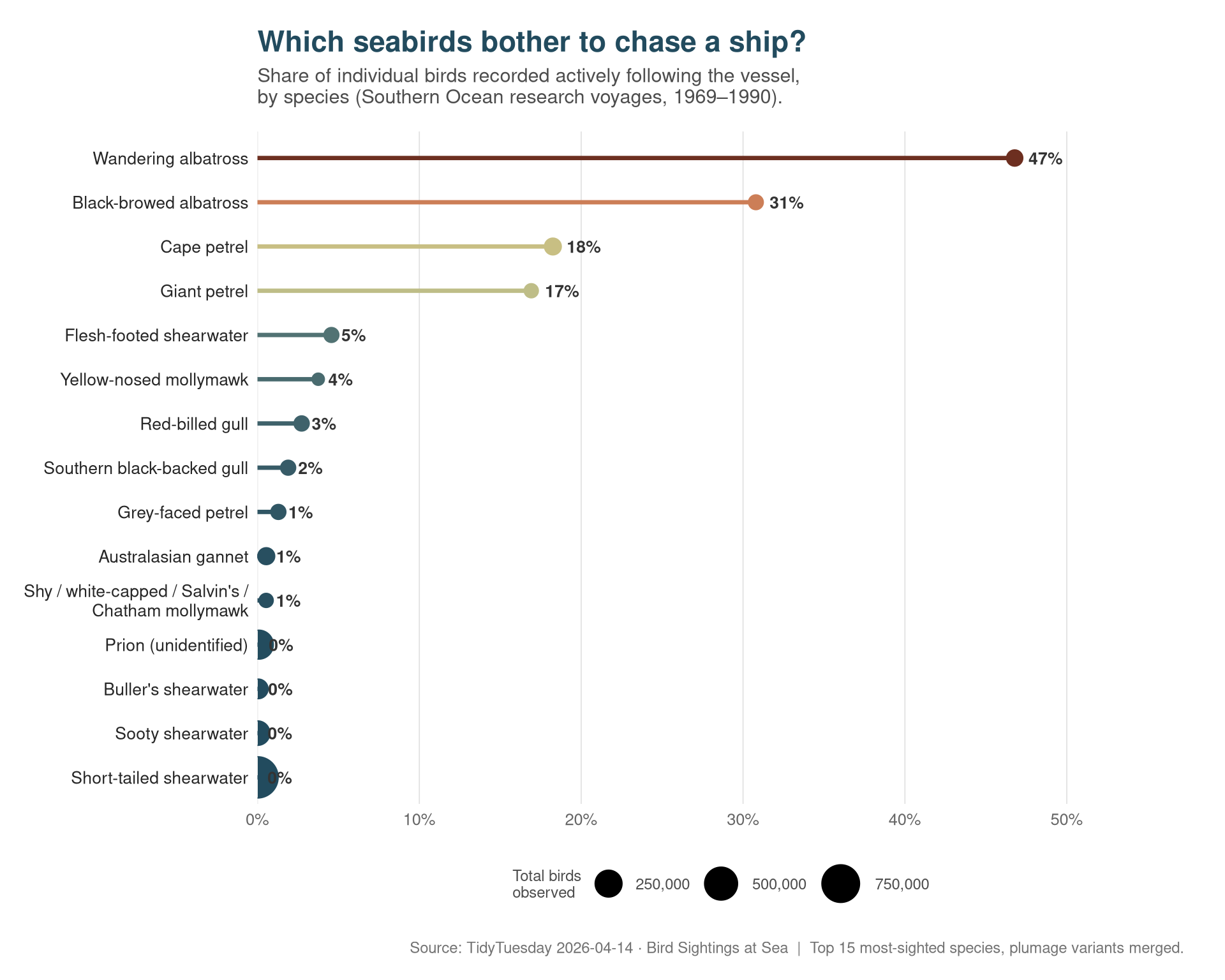
Final thoughts and takeaways
If you’ve ever stood on the stern rail of a ship south of New Zealand and watched a wandering albatross trail behind for the entire afternoon — never seeming to flap, just carving the air off the wake — this dataset will feel familiar. The number puts a percentage on the intuition: the wandering albatross spends most of its visible life behind boats, and so do the giant petrels and cape petrels that earn the old sailor’s name “Cape pigeon.” These are the obligate scavengers of the southern seas, and a ship is, to them, a feeding event in slow motion.
The shearwaters and the Australasian gannet sit at the opposite end of the same scale and are doing something different for a living: high-speed transit and plunge-diving on shoaling fish. A research vessel isn’t a buffet to them, it’s an obstacle to detour around.
A few caveats worth naming:
- The behavioral flags are observer-coded from the deck, and missingness is real — only about 57% of sightings carry a behavior code at all. The denominator I used (
total_birds) includes birds whose behavior wasn’t scored, so the percentages are conservative: the true rate of following-when-observed is higher. - “Following the ship” is partly a function of how slow you’re going. About 94% of the ship records are coded
steaming, sailing, but speed varies; a stationary research vessel deploying gear is more attractive than a freighter at 18 knots. - The dataset is historic (1969–1990). Several of the species in the top rank — especially the wandering and black-browed albatrosses — have suffered severe population declines from longline fishing bycatch in the decades since. The behavior that made them visible to these naturalists is the very same behavior that makes them vulnerable to baited hooks set astern.
The data tells one clean story and gestures at a darker one: the seabirds most willing to keep us company at sea are also the ones most exposed to the way we now fish it.