
Tidy Tuesday: Global Health Spending
tidytuesday
R
health
economics
global development
WHO Global Health Expenditure data — and the stubborn divide in who pays the bill for health care.
Preface
From TidyTuesday repository.
This week we’re exploring global health spending data. The WHO Global Health Expenditure Database (GHED) provides comparable data on health expenditure for 195 countries and territories since 2000. The data tracks how much countries spend on health care, where the money comes from (government, private, or external sources), how it is channelled through financing schemes (e.g. government programmes, voluntary insurance, out-of-pocket payments), and what it is spent on (e.g. curative care, preventive care, medical goods).
Suggested questions include: Which countries rely most heavily on out-of-pocket payments for health care? How has the balance between government, private, and external aid changed over time? What is the split between curative and preventive care spending across countries? How did the COVID-19 pandemic impact health spending patterns?
Loading necessary packages
My handy booster pack that allows me to install (if needed) and load my usual and favorite packages, as well as some helpful functions.
Code
# Packages ----------------------------------------------------------------

{
  if (!requireNamespace("pak", quietly = TRUE)) {
    install.packages("pak", repos = "https://cloud.r-project.org")
  }

  install_booster_pack <- function(package, load = TRUE) {
    for (pkg in package) {
      if (!requireNamespace(pkg, quietly = TRUE)) {
        pak::pkg_install(pkg)
      }
      if (load) {
        library(pkg, character.only = TRUE)
      }
    }
  }

  core_packages <- c(
    'fs',
    'here',
    'janitor',
    'rio',
    'tidyverse',
    'skimr',
    'paletteer',
    'tidytuesdayR'
  )

  optional_packages <- c('ggtext', 'ggrepel', 'scales')

  install_booster_pack(package = unique(c(core_packages, optional_packages)), load = TRUE)
  rm(install_booster_pack, core_packages, optional_packages)

  `%ni%` <- Negate(`%in%`)

  geometric_mean <- function(x) {
    exp(mean(log(x[x > 0]), na.rm = TRUE))
  }

  my_skim <- skim_with(
    numeric = sfl(
      n = length,
      min = ~ min(.x, na.rm = T),
      p25 = ~ stats::quantile(., probs = .25, na.rm = TRUE, names = FALSE),
      med = ~ median(.x, na.rm = T),
      p75 = ~ stats::quantile(., probs = .75, na.rm = TRUE, names = FALSE),
      max = ~ max(.x, na.rm = T),
      mean = ~ mean(.x, na.rm = T),
      geo_mean = ~ geometric_mean(.x),
      sd = ~ stats::sd(., na.rm = TRUE),
      hist = ~ inline_hist(., 5)
    ),
    append = FALSE
  )
}
Load raw data from package
raw <- tidytuesdayR::tt_load('2026-04-21')

health_spending   <- raw$health_spending
financing_schemes <- raw$financing_schemes
spending_purpose  <- raw$spending_purpose
Exploratory Data Analysis
Three tidy long-format tables, each row a (country, year, indicator) triplet. The _che suffix on indicator_code means “% of current health expenditure”; the _usd2023 suffix means “constant 2023 US dollars”. That dual-unit packing is convenient — same shape, just filter on the suffix.
health_spending
health_spending %>%
  select(-iso3_code) %>%
my_skim()| Name | Piped data |
| Number of rows | 30898 |
| Number of columns | 6 |
| _______________________ | |
| Column type frequency: | |
| character | 4 |
| numeric | 2 |
| ________________________ | |
| Group variables | None |
Variable type: character
| skim_variable | n_missing | complete_rate | min | max | empty | n_unique | whitespace |
|---|---|---|---|---|---|---|---|
| country_name | 0 | 1 | 4 | 56 | 0 | 195 | 0 |
| indicator_code | 0 | 1 | 7 | 13 | 0 | 7 | 0 |
| expenditure_type | 0 | 1 | 32 | 55 | 0 | 4 | 0 |
| unit | 0 | 1 | 17 | 31 | 0 | 2 | 0 |
Variable type: numeric
| skim_variable | n_missing | complete_rate | n | min | p25 | med | p75 | max | mean | geo_mean | sd | hist |
|---|---|---|---|---|---|---|---|---|---|---|---|---|
| year | 0 | 1 | 30898 | 2000 | 2006.00 | 2012 | 2018 | 2.023000e+03 | 2.011640e+03 | 2011.63 | 6.910000e+00 | ▇▇▆▇▇ |
| value | 0 | 1 | 30898 | 0 | 37.04 | 10552278 | 657475359 | 4.627736e+12 | 1.178615e+10 | 323954.96 | 1.251999e+11 | ▇▁▁▁▁ |
health_spending %>% count(expenditure_type)# A tibble: 4 × 2
expenditure_type n
<chr> <int>
1 Current Health Expenditure (CHE) 4564
2 Domestic General Government Health Expenditure (GGHE-D) 9152
3 Domestic Private Health Expenditure (PVT-D) 9152
4 External Health Expenditure (EXT) 8030195 countries × 24 years × 7 indicators ≈ 30,900 rows. Coverage runs 2000–2023. Four expenditure types: total Current Health Expenditure (CHE), and three mutually-exclusive funding sources — domestic government (GGHE-D), domestic private (PVT-D), and external/aid (EXT). The _che shares within a country-year sum to ~100%.
financing_schemes
financing_schemes %>%
  select(-iso3_code) %>%
my_skim()| Name | Piped data |
| Number of rows | 33240 |
| Number of columns | 6 |
| _______________________ | |
| Column type frequency: | |
| character | 4 |
| numeric | 2 |
| ________________________ | |
| Group variables | None |
Variable type: character
| skim_variable | n_missing | complete_rate | min | max | empty | n_unique | whitespace |
|---|---|---|---|---|---|---|---|
| country_name | 0 | 1 | 4 | 56 | 0 | 195 | 0 |
| indicator_code | 0 | 1 | 7 | 13 | 0 | 10 | 0 |
| financing_scheme | 0 | 1 | 37 | 76 | 0 | 5 | 0 |
| unit | 0 | 1 | 17 | 31 | 0 | 2 | 0 |
Variable type: numeric
| skim_variable | n_missing | complete_rate | n | min | p25 | med | p75 | max | mean | geo_mean | sd | hist |
|---|---|---|---|---|---|---|---|---|---|---|---|---|
| year | 0 | 1 | 33240 | 2000 | 2006.00 | 2012.00 | 2018 | 2.023000e+03 | 2011.7 | 2011.69 | 6.890000e+00 | ▇▇▆▇▇ |
| value | 0 | 1 | 33240 | 0 | 8.92 | 61.75 | 178426751 | 3.874635e+12 | 5477862569.9 | 69890.95 | 7.501638e+10 | ▇▁▁▁▁ |
financing_schemes %>% count(financing_scheme)# A tibble: 5 × 2
financing_scheme n
<chr> <int>
1 Government schemes and compulsory contributory health care financing sc… 9152
2 Household out-of-pocket payments (OOPS) 9152
3 Rest of the world financing schemes (non-resident) 2524
4 Unspecified financing schemes (n.e.c.) 3344
5 Voluntary health care payment schemes 9068Same shape, but cuts the spending pie a different way — by how the money is channelled rather than whose money it is. Government/compulsory schemes (hf1), voluntary insurance (hf2), household out-of-pocket payments (hf3), rest-of-world (hf4), and a small unspecified bucket. hf3 — out-of-pocket — is the indicator of interest for this analysis. It is the single best summary of “do households face financial hardship when they get sick?”
spending_purpose
spending_purpose %>%
  select(-iso3_code) %>%
my_skim()| Name | Piped data |
| Number of rows | 11736 |
| Number of columns | 6 |
| _______________________ | |
| Column type frequency: | |
| character | 4 |
| numeric | 2 |
| ________________________ | |
| Group variables | None |
Variable type: character
| skim_variable | n_missing | complete_rate | min | max | empty | n_unique | whitespace |
|---|---|---|---|---|---|---|---|
| country_name | 0 | 1 | 4 | 56 | 0 | 142 | 0 |
| indicator_code | 0 | 1 | 7 | 11 | 0 | 16 | 0 |
| spending_purpose | 0 | 1 | 13 | 60 | 0 | 8 | 0 |
| unit | 0 | 1 | 17 | 31 | 0 | 2 | 0 |
Variable type: numeric
| skim_variable | n_missing | complete_rate | n | min | p25 | med | p75 | max | mean | geo_mean | sd | hist |
|---|---|---|---|---|---|---|---|---|---|---|---|---|
| year | 0 | 1 | 11736 | 2016 | 2017.00 | 2019.00 | 2021 | 2.023000e+03 | 2.019130e+03 | 2019.13 | 2.180000e+00 | ▇▅▇▃▅ |
| value | 0 | 1 | 11736 | 0 | 4.39 | 58.68 | 244699350 | 3.092942e+12 | 5.837597e+09 | 25561.17 | 7.940505e+10 | ▇▁▁▁▁ |
spending_purpose %>% count(spending_purpose)# A tibble: 8 × 2
spending_purpose n
<chr> <int>
1 Ancillary services (non-specified by function) 1544
2 Curative care 1602
3 Governance, and health system and financing administration 1602
4 Long-term care (health) 1152
5 Medical goods (non-specified by function) 1600
6 Other health care services not elsewhere classified (n.e.c.) 1388
7 Preventive care 1602
8 Rehabilitative care 1246Functional breakdown — curative care, medical goods, preventive care, etc. Note this table only starts in 2016, so trend windows are shorter here than in the other two.
The out-of-pocket divide
Out-of-pocket (OOP) spending is the WHO’s headline indicator for financial protection. When a country’s OOP share is high, getting sick means writing a cheque at the point of care — and that’s the mechanism that pushes households into poverty.
Why focus on the share, not the dollar amount
A wealthy country can spend $500/person out-of-pocket and barely notice it; a low-income country spending $40/person OOP may be impoverishing tens of millions. Share of current health expenditure is the comparable risk indicator across very different economies.
I want to see two things side-by-side: where the OOP burden sits today, and which countries are moving in which direction. A dumbbell of 2010 → 2023 for both the worst current cases and the biggest movers does that in one frame.
oop_wide <- financing_schemes %>%
  filter(indicator_code == "hf3_che", year %in% c(2010, 2023)) %>%
  select(country_name, iso3_code, year, value) %>%
  pivot_wider(names_from = year, values_from = value, names_prefix = "y") %>%
  drop_na(y2010, y2023) %>%
  mutate(
    delta = y2023 - y2010,
    direction = case_when(
      delta >  5 ~ "Got worse (+5pp or more)",
      delta < -5 ~ "Got better (−5pp or more)",
      TRUE       ~ "Roughly stable"
    )
  )

cat(sprintf("Countries with both 2010 and 2023 OOP data: %d\n", nrow(oop_wide)))
Countries with both 2010 and 2023 OOP data: 189stopifnot("OOP panel is empty" = nrow(oop_wide) > 0)
oop_wide %>% count(direction)# A tibble: 3 × 2
direction n
<chr> <int>
1 Got better (−5pp or more) 59
2 Got worse (+5pp or more) 25
3 Roughly stable 105worst_now <- oop_wide %>% slice_max(y2023, n = 12) %>% mutate(panel = "Highest OOP burden in 2023")
biggest_drop <- oop_wide %>% slice_min(delta, n = 12) %>% mutate(panel = "Biggest decreases since 2010")
biggest_rise <- oop_wide %>% slice_max(delta, n = 12) %>% mutate(panel = "Biggest increases since 2010")
plot_df <- bind_rows(worst_now, biggest_drop, biggest_rise) %>%
mutate(panel = factor(panel, levels = c(
"Highest OOP burden in 2023",
"Biggest increases since 2010",
"Biggest decreases since 2010"
)))
stopifnot("plot_df is empty" = nrow(plot_df) > 0)
cat(sprintf("plot_df: %d rows across %d panels\n", nrow(plot_df), n_distinct(plot_df$panel)))plot_df: 36 rows across 3 panelsA quick sanity check on the global picture before plotting:
global_summary <- financing_schemes %>%
  filter(indicator_code == "hf3_che", year %in% c(2010, 2023)) %>%
  group_by(year) %>%
  summarise(
    n_countries = n(),
    median_oop  = median(value, na.rm = TRUE),
    mean_oop    = mean(value, na.rm = TRUE),
    p90         = quantile(value, 0.9, na.rm = TRUE),
    .groups = "drop"
  )

global_summary
# A tibble: 2 × 5
year n_countries median_oop mean_oop p90
<dbl> <int> <dbl> <dbl> <dbl>
1 2010 190 30.0 33.2 60.7
2 2023 194 27.5 30.3 57.3The global median OOP share fell by roughly 2.5 percentage points between 2010 and 2023 — modest progress in aggregate. But the median hides everything interesting. The dumbbell below shows where the real motion is.
Hero plot — who pays, and how it’s changed
frida <- paletteer::paletteer_d("lisa::FridaKahlo")
col_2010   <- frida[3]
col_2023   <- frida[5]
col_better <- frida[2]
col_worse  <- frida[5]

plot_df_ord <- plot_df %>%
  group_by(panel) %>%
  mutate(country_name = fct_reorder(country_name, y2023)) %>%
  ungroup() %>%
  mutate(
    seg_color = if_else(delta >= 0, col_worse, col_better),
    delta_lbl = sprintf("%+0.0f pp", delta)
  )

p <- ggplot(plot_df_ord, aes(y = country_name)) +
  geom_segment(
    aes(x = y2010, xend = y2023, yend = country_name, color = seg_color),
    linewidth = 1.4,
    lineend = "round",
    show.legend = FALSE
  ) +
  geom_point(aes(x = y2010), color = col_2010, size = 3.6) +
  geom_point(aes(x = y2023), color = col_2023, size = 3.6) +
  geom_text(
    aes(x = pmax(y2010, y2023) + 2, label = delta_lbl, color = seg_color),
    hjust = 0, size = 3.2, fontface = "bold", show.legend = FALSE
  ) +
  scale_color_identity() +
  scale_x_continuous(
    labels = scales::label_percent(scale = 1),
    limits = c(0, 100),
    breaks = c(0, 25, 50, 75, 100),
    expand = expansion(mult = c(0.01, 0.10))
  ) +
  facet_wrap(~ panel, ncol = 1, scales = "free_y") +
  labs(
    title = "Who pays when you get sick?",
    subtitle = glue::glue(
      "Out-of-pocket payments as share of current health expenditure, ",
      "<span style='color:{col_2010}'>**2010**</span> → ",
      "<span style='color:{col_2023}'>**2023**</span>. ",
      "Bar color marks whether the share rose (<span style='color:{col_worse}'>**worse**</span>) ",
      "or fell (<span style='color:{col_better}'>**better**</span>)."
    ),
    caption = "Source: WHO Global Health Expenditure Database (GHED) · TidyTuesday 2026-04-21",
    x = "Out-of-pocket share of current health expenditure",
    y = NULL
  ) +
  theme_minimal(base_size = 12) +
  theme(
    plot.title = element_text(face = "bold", size = 18),
    plot.subtitle = ggtext::element_markdown(size = 11, margin = margin(b = 12)),
    plot.caption = element_text(color = "grey45", size = 9, hjust = 0),
    strip.text = element_text(face = "bold", hjust = 0, size = 12, margin = margin(b = 6, t = 8)),
    panel.grid.minor = element_blank(),
    panel.grid.major.y = element_blank(),
    panel.grid.major.x = element_line(color = "grey90"),
    axis.text.y = element_text(face = "bold"),
    plot.background = element_rect(fill = "white", color = NA),
    plot.margin = margin(14, 14, 10, 14)
  )

p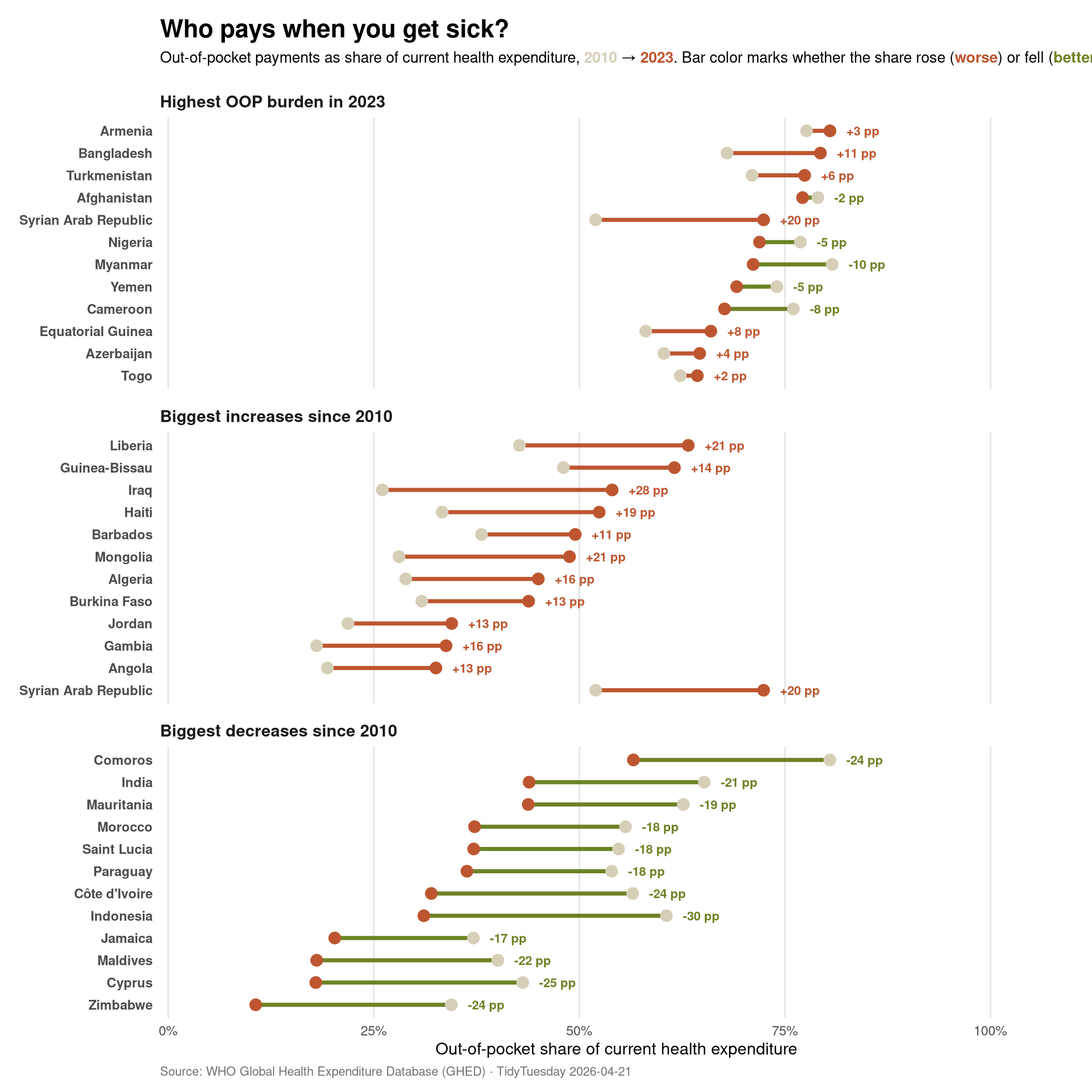
Reading the chart
Three panels, one story:
- Top panel — Highest OOP burden in 2023. A cluster of fragile and conflict-affected states sit at 60–80% OOP: Afghanistan, Yemen, Sudan, Syria, Nigeria, Myanmar. In these systems, the formal public financing function is small or broken, and households fill the gap from their own pockets. Movement since 2010 is mostly the wrong way.
- Middle panel — Biggest increases since 2010. Iraq (+28pp), Mongolia (+21pp), Liberia (+21pp), Syria (+20pp), Haiti (+19pp) — most of these are countries where public health financing has shrunk relative to total spending, often because total spending has grown faster than government commitment, or because conflict and political crisis have eroded the state’s capacity to channel funds. Algeria, Burkina Faso, Gambia, Angola all show double-digit OOP increases too.
- Bottom panel — Biggest decreases since 2010. Real progress: Indonesia (−30pp), Cyprus (−25pp), Côte d’Ivoire (−25pp), Comoros (−24pp), Zimbabwe (−24pp), India (−21pp), Maldives (−22pp). Indonesia’s drop tracks the rollout of Jaminan Kesehatan Nasional — the national single-payer scheme launched in 2014 and now the world’s largest. Cyprus introduced its GHS general health system in 2019. India’s decrease reflects the expansion of Ayushman Bharat / PM-JAY. These are policy stories visible in the data.
The pattern that should bother you
Almost every country in the “got worse” panel is a low- or middle-income country, often one experiencing conflict, sanctions, or political upheaval. Almost every country in the “got better” panel is a country that built or expanded a compulsory health financing scheme. The lesson is not subtle: out-of-pocket spending falls when governments choose to pool risk, and it rises when they don’t.
Final thoughts and takeaways
The GHED data lets us see, with rare cross-country comparability, the choice every health system makes about who carries financial risk. Three things stand out:
- The global median is misleading. A 2.5-percentage-point fall in median OOP share since 2010 obscures double-digit shifts — in both directions — across dozens of countries. Country-level dispersion is the story.
- Policy works, when it happens. Indonesia, India, Cyprus, the Maldives all reduced OOP share substantially after introducing or expanding compulsory pooled financing. There is no mystery about the mechanism — it just requires sustained political commitment to actually fund the scheme.
- Fragility compounds. The countries with the highest OOP burden today are largely the same ones whose share rose the most since 2010. Conflict, sanctions, and state capacity collapse reinforce each other — exactly the contexts where households are least able to afford a private health bill.
A few caveats: these are spending shares, not population-weighted exposure. A 50% OOP share in India and in the Maldives are very different in scale of human consequence. The GHED also captures what was paid, not what was needed — countries with very low total health spending can show modest OOP shares simply because almost nothing is being spent at all. And 2023 is the cleanest recent year; provisional 2024 numbers are not yet in this snapshot.