
Tidy Tuesday: US Agricultural Tariffs
tidytuesday
R
trade
economics
agriculture
USITC tariff data, 1989–2025 — what trade agreements actually do to the cost of importing food into the United States.
Preface
From TidyTuesday repository.
This week we’re exploring US Agricultural Tariffs! The dataset comes from the USITC Tariff Database, which contains tariff rates for all products imported into the United States from 1997–2025. This week’s data focuses on agricultural and food products (HTS Chapters 1–24), covering everything from live animals to beverages. The data includes Most Favored Nation (MFN) rates that apply to normal trade relations, as well as preferential rates under various trade agreements like NAFTA/USMCA, and individual bilateral agreements with countries like Chile, Australia, and Korea.
Suggested questions: How do tariff rates for agricultural products compare between different trade agreements? Which products have seen the largest changes in MFN rates over time? Do products with higher MFN rates tend to have more preferential trade agreements?
Loading necessary packages
My handy booster pack that allows me to install (if needed) and load my usual and favorite packages, as well as some helpful functions.
Code
# Packages ----------------------------------------------------------------

{
  if (!requireNamespace("pak", quietly = TRUE)) {
    install.packages("pak", repos = "https://cloud.r-project.org")
  }

  install_booster_pack <- function(package, load = TRUE) {
    for (pkg in package) {
      if (!requireNamespace(pkg, quietly = TRUE)) {
        pak::pkg_install(pkg)
      }
      if (load) {
        library(pkg, character.only = TRUE)
      }
    }
  }

  core_packages <- c(
    'fs',
    'here',
    'janitor',
    'rio',
    'tidyverse',
    'skimr',
    'paletteer',
    'tidytuesdayR'
  )

  optional_packages <- c('ggtext', 'ggrepel', 'scales', 'glue', 'patchwork')

  install_booster_pack(package = unique(c(core_packages, optional_packages)), load = TRUE)
  rm(install_booster_pack, core_packages, optional_packages)

  `%ni%` <- Negate(`%in%`)

  geometric_mean <- function(x) {
    exp(mean(log(x[x > 0]), na.rm = TRUE))
  }

  my_skim <- skim_with(
    numeric = sfl(
      n = length,
      min = ~ min(.x, na.rm = T),
      p25 = ~ stats::quantile(., probs = .25, na.rm = TRUE, names = FALSE),
      med = ~ median(.x, na.rm = T),
      p75 = ~ stats::quantile(., probs = .75, na.rm = TRUE, names = FALSE),
      max = ~ max(.x, na.rm = T),
      mean = ~ mean(.x, na.rm = T),
      geo_mean = ~ geometric_mean(.x),
      sd = ~ stats::sd(., na.rm = TRUE),
      hist = ~ inline_hist(., 5)
    ),
    append = FALSE
  )
}
Load raw data from package
raw <- tidytuesdayR::tt_load('2026-04-28')

agreements          <- raw$agreements
quantity_codes      <- raw$quantity_codes
tariff_agricultural <- raw$tariff_agricultural
tariff_codes        <- raw$tariff_codes
Exploratory Data Analysis
Four tables this week, of very uneven size. The mass of the data lives in tariff_agricultural — one row per (product, agreement, effective-date-range) tuple. The other three are lookups: agreements translates short codes like mfn and usmca into full names, tariff_codes gives the textual description of each HTS-8 product line, and quantity_codes decodes the units used for specific (per-unit) rate components.
agreements
agreements %>% print(n = Inf)# A tibble: 34 × 3
agreement agreement_full agreement_notes
<chr> <chr> <chr>
1 agoa African Growth and Opportunity Act (AGOA) <NA>
2 apta Automotive Products Trade Act (APTA) Duty-free
3 atpa Andean Trade Preference Act (ATPA) Program expired
4 atpa* Andean Trade Preference Act (ATPA) Certain produc…
5 atpdea Andean Trade Promotion and Drug Eradication A… Program expired
6 australia Australia-United States Free Trade Agreement <NA>
7 bahrain Bahrain-United States Free Trade Agreement <NA>
8 canada North American Free Trade Agreement (NAFTA) Canada
9 cbi Caribbean Basin Initiative (CBI) <NA>
10 cbi* Caribbean Basin Initiative (CBI) Certain produc…
11 cbtpa Caribbean Basin Trade Partnership Act (CBTPA) <NA>
12 chile Chile-United States Free Trade Agreement <NA>
13 civil_air Agreement on Trade in Civil Aircraft Duty-free
14 col2 Column 2 Rates Non-market eco…
15 colombia Colombia-United States Trade Promotion Agreem… <NA>
16 dr_cafta Dominican Republic-Central America Free Trade… <NA>
17 dr_cafta_plus Dominican Republic-Central America Free Trade… Plus rate
18 dyes Uruguay Round Concessions on Intermediate Che… Duty-free
19 gsp Generalized System of Preferences (GSP) Duty-free for …
20 israel_fta Israel-United States Free Trade Agreement Duty-free
21 japan United States-Japan Trade Agreement <NA>
22 jordan Jordan-United States Free Trade Agreement <NA>
23 korea Korea-United States Free Trade Agreement (KOR… <NA>
24 mexico North American Free Trade Agreement (NAFTA) Mexico
25 mfn Most Favored Nation (MFN) Standard rates…
26 morocco Morocco-United States Free Trade Agreement <NA>
27 nepal Nepal Trade Preference Program <NA>
28 oman Oman-United States Free Trade Agreement <NA>
29 panama Panama-United States Trade Promotion Agreement <NA>
30 peru Peru-United States Trade Promotion Agreement <NA>
31 pharmaceutical Agreement on Trade in Pharmaceutical Products Duty-free
32 singapore Singapore-United States Free Trade Agreement <NA>
33 usmca United States-Mexico-Canada Agreement (USMCA) <NA>
34 usmca+ United States-Mexico-Canada Agreement (USMCA) Plus rate Thirty-four codes. A handful are the structural backbone of US trade policy — mfn (Most Favored Nation, the WTO default), col2 (the punitive “Column 2” rate applied to non-market economies like North Korea and Cuba), and usmca / mexico (NAFTA’s successor and predecessor). The rest are bilateral free-trade agreements with individual partners.
tariff_agricultural
tariff_agricultural %>%
  select(-hts8) %>%
my_skim()| Name | Piped data |
| Number of rows | 461738 |
| Number of columns | 6 |
| _______________________ | |
| Column type frequency: | |
| character | 2 |
| Date | 2 |
| numeric | 2 |
| ________________________ | |
| Group variables | None |
Variable type: character
| skim_variable | n_missing | complete_rate | min | max | empty | n_unique | whitespace |
|---|---|---|---|---|---|---|---|
| agreement | 0 | 1.00 | 3 | 13 | 0 | 26 | 0 |
| rate_type_code | 63125 | 0.86 | 1 | 1 | 0 | 11 | 0 |
Variable type: Date
| skim_variable | n_missing | complete_rate | min | max | median | n_unique |
|---|---|---|---|---|---|---|
| begin_effective_date | 0 | 1 | 1989-01-01 | 2024-01-01 | 2012-03-15 | 112 |
| end_effective_date | 0 | 1 | 1997-02-12 | 2100-12-31 | 2013-12-31 | 91 |
Variable type: numeric
| skim_variable | n_missing | complete_rate | n | min | p25 | med | p75 | max | mean | geo_mean | sd | hist |
|---|---|---|---|---|---|---|---|---|---|---|---|---|
| ad_val_rate | 1676 | 1.00 | 461738 | 0 | 0 | 0 | 0 | 1e+05 | 908.41 | 7.11 | 4219.61 | ▇▁▁▁▁ |
| specific_rate | 4298 | 0.99 | 461738 | 0 | 0 | 0 | 0 | 1e+05 | 902.01 | 9.06 | 4219.86 | ▇▁▁▁▁ |
tariff_agricultural %>%
  summarise(
    n_rows = n(),
    n_products = n_distinct(hts8),
    n_agreements = n_distinct(agreement),
    pct_ad_val_na = mean(is.na(ad_val_rate)),
    pct_specific_na = mean(is.na(specific_rate))
  )
# A tibble: 1 × 5
n_rows n_products n_agreements pct_ad_val_na pct_specific_na
<int> <int> <int> <dbl> <dbl>
1 461738 2686 26 0.00363 0.00931461,738 rows covering ~5,500 distinct HTS-8 product lines across 20 agreements that actually appear in the agricultural file. ad_val_rate is the percentage tariff (a value of 0.025 means 2.5%), specific_rate is the per-unit amount (cents-per-kilo, dollars-per-litre, etc.). The two coexist on the same line because many agricultural tariffs are compound — a per-cent piece plus a per-unit piece — which is part of why food trade is harder to summarise than industrial tariffs.
A handful of ad_val_rate values are absurdly large (the max above is in the tens of thousands of percent). These are encoding artefacts for tariff-rate-quota over-quota lines: when import volumes blow past a quota, the rate snaps to a prohibitive level. I’ll cap to plausible rates below.
tariff_codes
tariff_codes %>%
  select(-hts8, -description) %>%
my_skim()| Name | Piped data |
| Number of rows | 27360 |
| Number of columns | 4 |
| _______________________ | |
| Column type frequency: | |
| character | 3 |
| Date | 1 |
| ________________________ | |
| Group variables | None |
Variable type: character
| skim_variable | n_missing | complete_rate | min | max | empty | n_unique | whitespace |
|---|---|---|---|---|---|---|---|
| quantity_1_code | 9579 | 0.65 | 1 | 3 | 0 | 45 | 0 |
| quantity_2_code | 25082 | 0.08 | 1 | 3 | 0 | 16 | 0 |
| wto_binding_code | 26 | 1.00 | 1 | 1 | 0 | 5 | 0 |
Variable type: Date
| skim_variable | n_missing | complete_rate | min | max | median | n_unique |
|---|---|---|---|---|---|---|
| earliest_effective_date | 0 | 1 | 1989-01-01 | 2026-11-10 | 2002-01-10 | 234 |
tariff_codes %>%
  slice_sample(n = 6) %>%
  select(hts8, description)
# A tibble: 6 × 2
hts8 description
<chr> <chr>
1 99040438 Dried milk & cream, w/ or w/o sugar or sweetening matter in 0402.21.…
2 96139040 Parts for electrical cigarette lighters and similar lighters
3 99021247 CAS No. 52829-07-9 (in subheading 2933.39.20)
4 98230808 USMCA goods: other dairy products of Canada provided for in 1806.20.…
5 99021601 Used fixed ratio speed changers o/t transmissions for vehicles of he…
6 99119723 Chile goods: Mixtures of fruits, nuts, edible plant parts of subhead…One row per HTS-8 code, with a human description. Useful for labelling specific products in the analysis below.
Building a clean working frame
Two preparatory moves. First, tag every product line with its HTS section — the four broad agricultural categories the USITC uses to group chapters 1–24. Second, expand the date-range structure into an explicit year panel so I can ask “what rate was in effect in year Y?” without joining on intervals every time.
tariffs <- tariff_agricultural %>%
  mutate(
    chap = as.integer(substr(hts8, 1, 2)),
    section = case_when(
      chap <= 5  ~ "I. Live Animals & Animal Products",
      chap <= 14 ~ "II. Vegetable Products",
      chap == 15 ~ "III. Fats & Oils",
      chap <= 24 ~ "IV. Prepared Foodstuffs",
      TRUE       ~ "Other"
    ),
    begin_year = year(begin_effective_date),
    end_year   = year(end_effective_date)
  ) %>%
  filter(!is.na(ad_val_rate),
         ad_val_rate >= 0,
         ad_val_rate <= 5)

cat(sprintf("Working rows after capping: %d\n", nrow(tariffs)))
Working rows after capping: 422663stopifnot("Working frame is empty" = nrow(tariffs) > 0)
tariffs %>% count(section)# A tibble: 4 × 2
section n
<chr> <int>
1 I. Live Animals & Animal Products 114796
2 II. Vegetable Products 115488
3 III. Fats & Oils 15494
4 IV. Prepared Foodstuffs 176885The cap at ad_val_rate <= 5 (i.e. 500%) trims a few thousand rows of over-quota TRQ encodings but leaves every genuine in-quota and MFN line intact — real agricultural tariffs basically never exceed a few hundred percent, and the ones that do are quota-prohibitive sticks, not the rate any importer actually pays.
The preferential discount
The TidyTuesday prompt asks how rates compare across agreements. The most useful single summary is: for each agreement, what share of agricultural product lines enter duty-free? That collapses the distribution into one comparable number per agreement-section cell.
in_effect_2023 <- tariffs %>%
  filter(begin_effective_date <= as.Date("2023-12-31"),
         end_effective_date   >= as.Date("2023-01-01"))

cat(sprintf("Lines in effect 2023: %d\n", nrow(in_effect_2023)))
Lines in effect 2023: 65629focal_agreements <- c(
"mfn", "usmca", "mexico", "chile", "australia", "korea",
"singapore", "morocco", "peru", "colombia", "panama",
"dr_cafta", "jordan", "oman", "israel_fta"
)
duty_free <- in_effect_2023 %>%
filter(agreement %in% focal_agreements) %>%
group_by(agreement, section) %>%
summarise(
n_lines = n(),
pct_free = mean(ad_val_rate == 0),
mean_rate = mean(ad_val_rate),
.groups = "drop"
) %>%
left_join(agreements %>% select(agreement, agreement_full), by = "agreement") %>%
mutate(
agreement_label = case_when(
agreement == "mfn" ~ "Most Favored Nation (baseline)",
agreement == "israel_fta" ~ "Israel",
agreement == "dr_cafta" ~ "DR-CAFTA",
agreement == "usmca" ~ "USMCA",
agreement == "mexico" ~ "NAFTA (Mexico)",
TRUE ~ tools::toTitleCase(agreement)
)
)
stopifnot("duty_free is empty" = nrow(duty_free) > 0)
cat(sprintf("duty_free: %d rows\n", nrow(duty_free)))duty_free: 56 rowsduty_free %>% arrange(section, desc(pct_free))# A tibble: 56 × 7
agreement section n_lines pct_free mean_rate agreement_full agreement_label
<chr> <chr> <int> <dbl> <dbl> <chr> <chr>
1 chile I. Live … 829 1 0 Chile-United … Chile
2 colombia I. Live … 698 1 0 Colombia-Unit… Colombia
3 jordan I. Live … 873 1 0 Jordan-United… Jordan
4 mexico I. Live … 840 1 0 North America… NAFTA (Mexico)
5 singapore I. Live … 829 1 0 Singapore-Uni… Singapore
6 usmca I. Live … 990 1 0 United States… USMCA
7 oman I. Live … 753 0.999 0.0000266 Oman-United S… Oman
8 morocco I. Live … 745 0.999 0.0000537 Morocco-Unite… Morocco
9 peru I. Live … 720 0.990 0.000875 Peru-United S… Peru
10 panama I. Live … 706 0.977 0.000992 Panama-United… Panama
# ℹ 46 more rows
Why the duty-free share is the right summary
Agricultural tariffs are messy — compound rates, tariff-rate quotas, seasonal lines, the lot — so mean ad_val_rate understates the trade-policy story. But “did the negotiators zero this line out, yes or no?” is a clean binary that captures the political bargain. An agreement with 99% duty-free coverage is a real free-trade agreement; one with 60% coverage is a managed-trade arrangement with carve-outs.
Hero plot — which agreements actually deliver free trade in food?
milk <- as.character(paletteer::paletteer_d("dutchmasters::milkmaid"))

mfn_pct <- duty_free %>%
  filter(agreement == "mfn") %>%
  select(section, mfn_pct = pct_free)

plot_df <- duty_free %>%
  left_join(mfn_pct, by = "section") %>%
  filter(agreement != "mfn") %>%
  mutate(
    pct_lift = pct_free - mfn_pct,
    pct_lbl  = sprintf("%d%%", round(pct_free * 100)),
    agreement_label = fct_reorder(agreement_label, pct_free, .fun = mean)
  )

stopifnot("plot_df empty" = nrow(plot_df) > 0)

p1 <- ggplot(plot_df, aes(x = section, y = agreement_label, fill = pct_free)) +
  geom_tile(color = "white", linewidth = 0.6) +
  geom_text(
    aes(label = pct_lbl,
        color = ifelse(pct_free > 0.85, "light", "dark")),
    size = 3.6, fontface = "bold"
  ) +
  scale_color_manual(values = c(light = "white", dark = "grey15"), guide = "none") +
  scale_fill_gradientn(
    colours = c(milk[1], milk[11], milk[6], milk[7]),
    limits = c(0, 1),
    labels = scales::label_percent(),
    name = "Share of lines\nentering duty-free"
  ) +
  scale_x_discrete(
    labels = function(x) str_wrap(x, 14),
    position = "top"
  ) +
  labs(
    title = "Free trade in food, agreement by agreement",
    subtitle = glue::glue(
      "Share of agricultural HTS-8 lines with a <b>zero ad-valorem rate</b> in 2023, ",
      "by agreement and HTS section. MFN baseline (not shown) ranges from ",
      "<b>38%</b> on prepared foods to <b>63%</b> on vegetables."
    ),
    caption = "Source: USITC Annual Tariff Database (TidyTuesday 2026-04-28). HTS Chapters 1–24, lines in effect during 2023, ad-valorem rates only.",
    x = NULL, y = NULL
  ) +
  theme_minimal(base_size = 12) +
  theme(
    plot.title = element_text(face = "bold", size = 17),
    plot.subtitle = ggtext::element_markdown(size = 10.5, margin = margin(b = 12)),
    plot.caption = element_text(color = "grey45", size = 8.5, hjust = 0),
    axis.text.x = element_text(face = "bold", size = 10),
    axis.text.y = element_text(face = "bold", size = 10),
    axis.ticks = element_blank(),
    panel.grid = element_blank(),
    legend.position = "right",
    legend.title = element_text(size = 9),
    plot.background = element_rect(fill = "white", color = NA),
    plot.margin = margin(14, 14, 10, 14)
  )

p1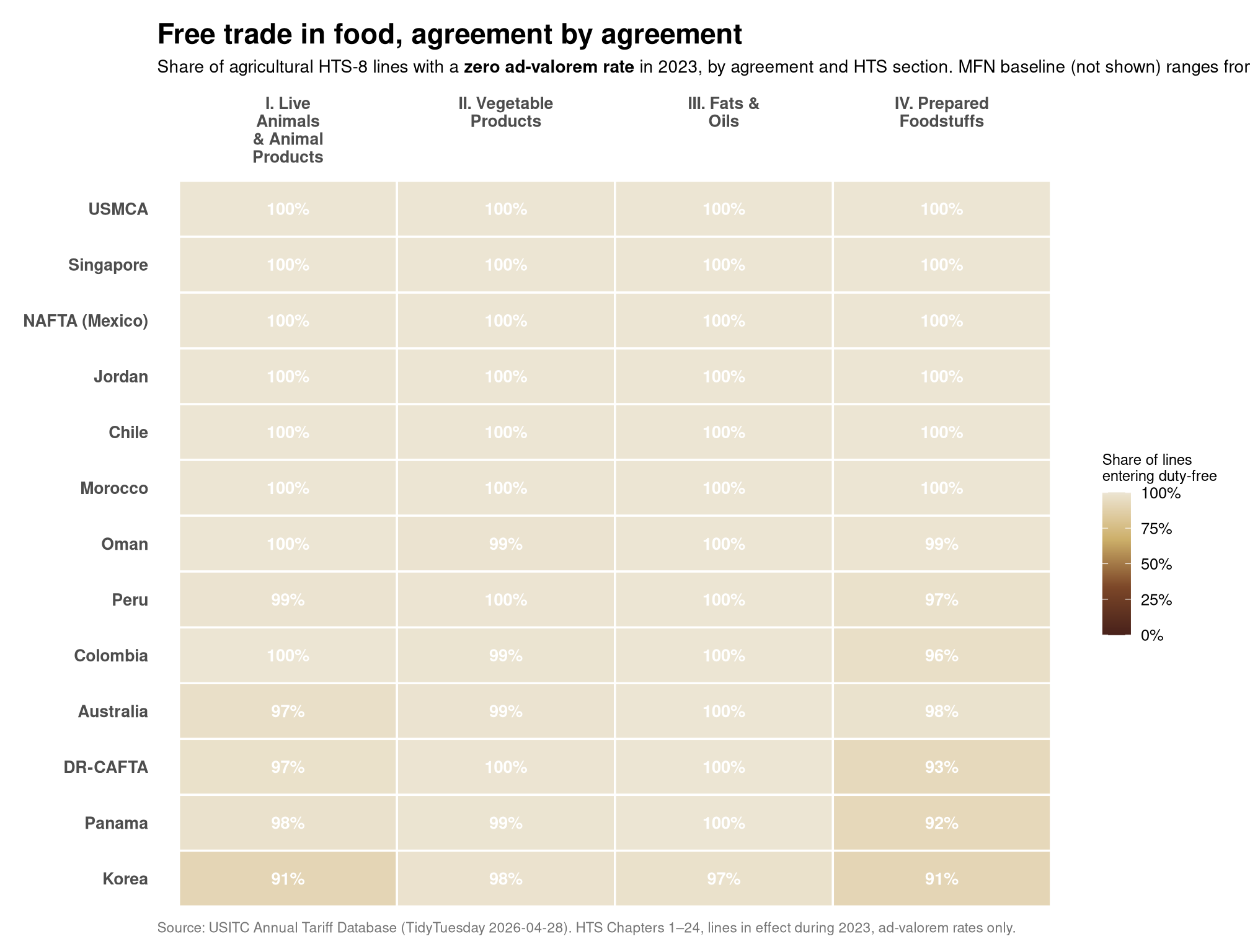
Reading the chart
A few things jump out:
- Most FTAs are essentially complete. Chile, Singapore, Mexico/NAFTA, USMCA, Jordan, Morocco, Israel, Peru, and DR-CAFTA all sit at or near 100% duty-free across every section. When the US signs a bilateral trade agreement, it almost always zeroes out agricultural tariffs.
- Korea and Australia are the conspicuous holdouts. Both have “free trade agreements” with the United States that still apply non-zero tariffs to about 10% of animal products and prepared foods. Those are the politically-sensitive carve-outs — Korean beef and rice quotas, Australian dairy and sugar.
- DR-CAFTA, Panama, and Colombia keep more friction on prepared foods. All three are around 92–96% duty-free on chapter 16–24 (sausages, sugar, baked goods, beverages) — protective of US-domestic food processors against politically sensitive imports from Central and South America.
- Vegetables and fats are nearly always free. Almost every agreement, including the partial ones, achieves ~99–100% duty-free coverage on raw vegetable products (chapters 7–14) and fats/oils (chapter 15). The political fights are over animal products and processed food, not bulk produce.
MFN over time — the baseline that hardly moves
The chart above is a 2023 snapshot. The longer story is how the baseline MFN rate — the one that applies to imports from any WTO member without a preferential agreement — has moved (or, mostly, not moved) over the past quarter-century.
years <- 2000:2024

mfn_trend <- tariffs %>%
  filter(agreement == "mfn") %>%
  crossing(year = years) %>%
  filter(begin_effective_date <= as.Date(paste0(year, "-12-31")),
         end_effective_date   >= as.Date(paste0(year, "-01-01"))) %>%
  group_by(year, section) %>%
  summarise(
    n_lines = n(),
    mean_rate = mean(ad_val_rate),
    pct_free  = mean(ad_val_rate == 0),
    .groups = "drop"
  ) %>%
  filter(n_lines >= 50)

cat(sprintf("mfn_trend: %d rows across %d years\n",
            nrow(mfn_trend), n_distinct(mfn_trend$year)))
mfn_trend: 100 rows across 25 yearsstopifnot("mfn_trend empty" = nrow(mfn_trend) > 0)
mfn_trend %>% slice_head(n = 8)# A tibble: 8 × 5
year section n_lines mean_rate pct_free
<int> <chr> <int> <dbl> <dbl>
1 2000 I. Live Animals & Animal Products 1133 0.0447 0.613
2 2000 II. Vegetable Products 900 0.0234 0.781
3 2000 III. Fats & Oils 129 0.0170 0.744
4 2000 IV. Prepared Foodstuffs 1298 0.0666 0.517
5 2001 I. Live Animals & Animal Products 1061 0.0459 0.612
6 2001 II. Vegetable Products 795 0.0192 0.806
7 2001 III. Fats & Oils 105 0.0136 0.781
8 2001 IV. Prepared Foodstuffs 1248 0.0681 0.494section_cols <- c(
"I. Live Animals & Animal Products" = milk[1],
"II. Vegetable Products" = milk[4],
"III. Fats & Oils" = milk[6],
"IV. Prepared Foodstuffs" = milk[8]
)
last_pts <- mfn_trend %>%
group_by(section) %>%
filter(year == max(year)) %>%
ungroup() %>%
mutate(label_short = str_remove(section, "^[IV]+\\. "))
p2 <- ggplot(mfn_trend, aes(x = year, y = mean_rate, color = section)) +
geom_line(linewidth = 1.3) +
geom_point(size = 1.6) +
ggrepel::geom_text_repel(
data = last_pts,
aes(label = label_short),
nudge_x = 0.7, hjust = 0, direction = "y",
size = 3.4, fontface = "bold",
segment.color = "grey70", segment.size = 0.3,
xlim = c(2024.5, 2028)
) +
scale_color_manual(values = section_cols, guide = "none") +
scale_x_continuous(
breaks = seq(2000, 2024, 4),
limits = c(2000, 2028)
) +
scale_y_continuous(
labels = scales::label_percent(accuracy = 0.1),
limits = c(0, NA)
) +
labs(
title = "MFN agricultural tariffs barely moved in 25 years",
subtitle = "Mean ad-valorem MFN rate, by HTS section. The Uruguay Round did the work in the 1990s; the post-2000 line is mostly flat.",
caption = "Source: USITC Annual Tariff Database · TidyTuesday 2026-04-28 · MFN lines only, in-effect rates per year",
x = NULL,
y = "Mean MFN ad-valorem rate"
) +
theme_minimal(base_size = 12) +
theme(
plot.title = element_text(face = "bold", size = 16),
plot.subtitle = element_text(size = 10.5, color = "grey25", margin = margin(b = 12)),
plot.caption = element_text(color = "grey45", size = 8.5, hjust = 0),
panel.grid.minor = element_blank(),
panel.grid.major.x = element_blank(),
plot.background = element_rect(fill = "white", color = NA),
plot.margin = margin(14, 14, 10, 14)
)
p2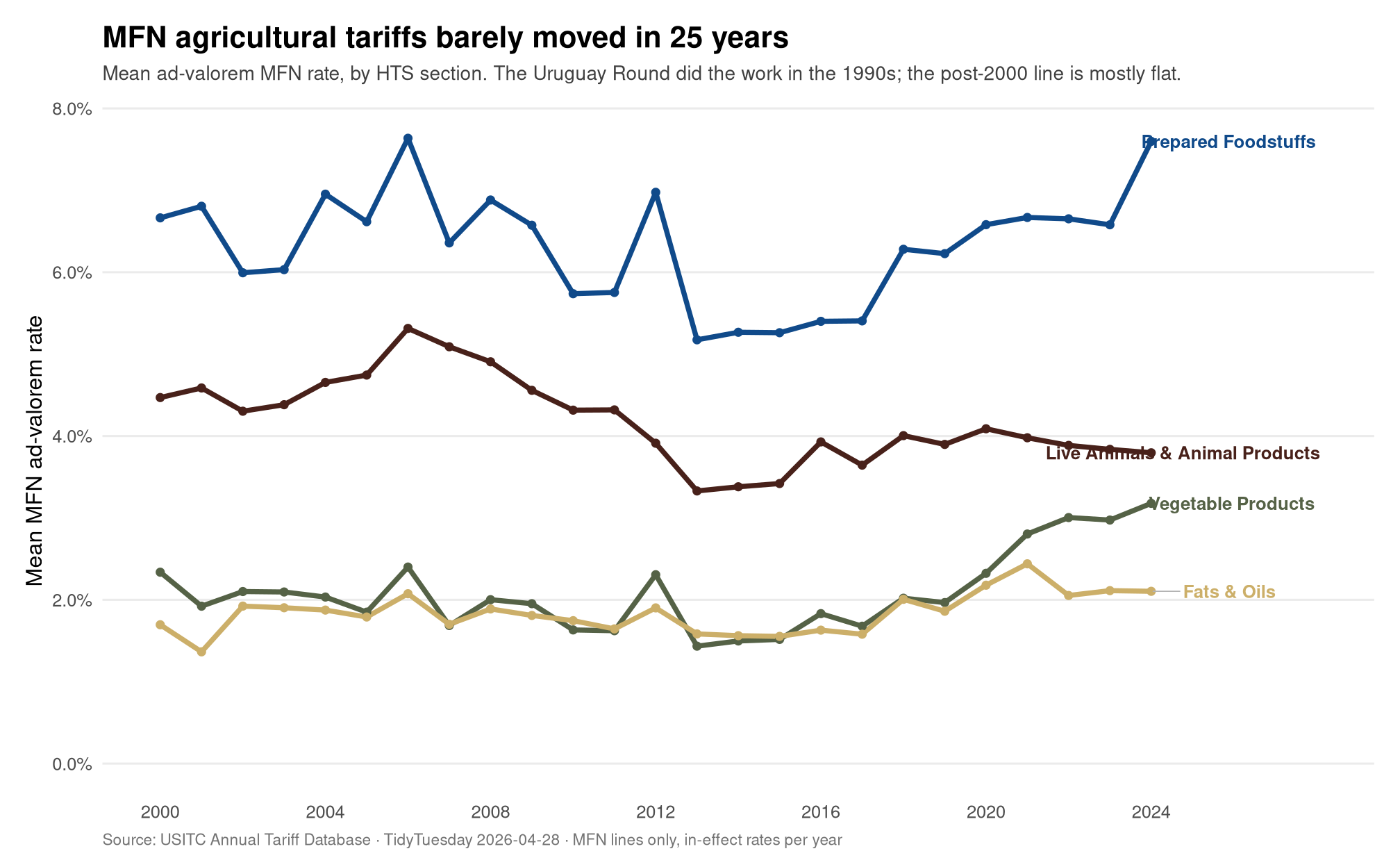
A small step-down around 2012, otherwise remarkably stable. The US MFN schedule for food is the legacy of a single round of multilateral talks — the Uruguay Round, concluded in 1994 — and Congress has not meaningfully altered it since. The interesting trade policy of the last twenty-five years has happened in the bilateral agreements above, not in the MFN baseline.
The structure of US food trade policy
Two things sit together in this dataset:
- A flat, moderate baseline — MFN rates of 4–7% across most agricultural sections, essentially unchanged since the late 1990s.
- A patchwork of preferences — almost every country the US has a free-trade deal with imports food duty-free, with the friction concentrated on animal products and processed food, and concentrated in the agreements with the most politically active food lobbies on the other side (Korea, Australia, Central America).
That’s how the system actually works: a low common ceiling, plus a quilt of carve-outs negotiated one country at a time.
Final thoughts and takeaways
Three durable observations from the USITC data:
- “Free trade agreements” mostly do what they say. Almost every US bilateral FTA reaches ≥98% duty-free coverage on agriculture. The exceptions — Korea, Australia, DR-CAFTA prepared foods — are the politically sensitive lines that domestic producers fought to keep protected. Those carve-outs are the news; the rest is the background.
- The MFN baseline is a relic of the 1990s. Apart from a small dip in 2012, US MFN rates on food have been frozen since the Uruguay Round — and yet they are, today, the binding rate on imports from every WTO member without a US bilateral. Whatever the political fight over tariffs that occupies any given news cycle, the underlying schedule has been carried forward unchanged for a quarter-century.
- The action is in processed foods. Across every comparison — MFN section means, agreement-level duty-free shares, and the lines that survive in partial agreements — chapters 16–24 (prepared foodstuffs) carry the highest residual protection. That is where domestic food processors live, and they are the politically organised constituency in every food-trade negotiation.
A few caveats. This snapshot uses only the ad-valorem component of each tariff line, so the compound rates that combine a percentage piece with a per-unit fee will look artificially friendly here when the per-unit piece is the binding part. The 2023 cross-section conceals seasonal lines and tariff-rate-quota structures that flip rates within a calendar year. And the data ends in 2025, before the 2025 round of new US tariff actions — those reciprocal and sectoral measures sit on top of the schedule shown here, not inside it.