Tidy Tuesday: Italian Industrial Production
tidytuesday
R
history
economics
Italy
One hundred and twenty years of Italian industrialization — reading war, recovery, and the economic miracle through production records.
Preface
From TidyTuesday repository.
This week we’re exploring Italian Industrial Production. The dataset comes from “A monetray history of Italy” by Fratianni and Spinelli (1997), via the GESIS Data Archive (ZA8700). It contains data on Italian industrial production covering food and beverages, textiles, and transport manufacturing spanning from 1861 through 1985 — a 124-year window that encompasses Italian unification, two world wars, fascism, and the postwar economic miracle.
The three tables — food_beverages, textiles, and transport — share a common integer year axis but start at different points and carry heavy missing data in the early decades before those industries were formally tracked. The analytical question this post pursues: how does wartime disruption and the postwar recovery show up simultaneously across three distinct industrial sectors?
Loading necessary packages
Code
{
  if (!requireNamespace("pak", quietly = TRUE)) {
    install.packages("pak", repos = "https://cloud.r-project.org")
  }

  install_booster_pack <- function(package, load = TRUE) {
    for (pkg in package) {
      if (!requireNamespace(pkg, quietly = TRUE)) {
        pak::pkg_install(pkg)
      }
      if (load) {
        library(pkg, character.only = TRUE)
      }
    }
  }

  core_packages <- c(
    'fs', 'here', 'janitor', 'rio',
    'tidyverse', 'skimr', 'paletteer', 'tidytuesdayR'
  )

  optional_packages <- c('ggtext', 'ggrepel', 'scales', 'patchwork')

  install_booster_pack(package = unique(c(core_packages, optional_packages)), load = TRUE)
  rm(install_booster_pack, core_packages, optional_packages)

  `%ni%` <- Negate(`%in%`)

  geometric_mean <- function(x) {
    exp(mean(log(x[x > 0]), na.rm = TRUE))
  }

  my_skim <- skim_with(
    numeric = sfl(
      n = length,
      min = ~ min(.x, na.rm = T),
      p25 = ~ stats::quantile(., probs = .25, na.rm = TRUE, names = FALSE),
      med = ~ median(.x, na.rm = T),
      p75 = ~ stats::quantile(., probs = .75, na.rm = TRUE, names = FALSE),
      max = ~ max(.x, na.rm = T),
      mean = ~ mean(.x, na.rm = T),
      geo_mean = ~ geometric_mean(.x),
      sd = ~ stats::sd(., na.rm = TRUE),
      hist = ~ inline_hist(., 5)
    ),
    append = FALSE
  )
}
Load raw data from package
raw <- tidytuesdayR::tt_load('2026-05-05')

food_beverages <- raw$food_beverages
textiles       <- raw$textiles
transport      <- raw$transport
Exploratory Data Analysis
The my_skim() function is a modified version of the skimr::skim() function that returns the number of missing data points (cells as NA) as well as the inverse (e.g.: number of rows that are not NA), the count, minimum, 25%, median, 75%, max, mean, geometric mean, and standard deviation. It also generates a little ASCII histogram. Neat!
food_beverages
my_skim(food_beverages)| Name | food_beverages |
| Number of rows | 115 |
| Number of columns | 8 |
| _______________________ | |
| Column type frequency: | |
| numeric | 8 |
| ________________________ | |
| Group variables | None |
Variable type: numeric
| skim_variable | n_missing | complete_rate | n | min | p25 | med | p75 | max | mean | geo_mean | sd | hist |
|---|---|---|---|---|---|---|---|---|---|---|---|---|
| Year | 0 | 1.00 | 115 | 1871 | 1899.50 | 1928.0 | 1956.5 | 1985 | 1928.00 | 1927.71 | 33.34 | ▇▇▇▇▇ |
| Sugar | 7 | 0.94 | 115 | 19 | 77360.75 | 295597.5 | 906615.8 | 2011316 | 489144.37 | 99727.93 | 516624.03 | ▇▂▂▁▁ |
| Glucose | 17 | 0.85 | 115 | 4754 | 43246.00 | 94112.5 | 428403.8 | 2223565 | 357468.94 | 132832.33 | 533728.82 | ▇▁▁▁▁ |
| Coffee_substitute | 18 | 0.84 | 115 | 87 | 28622.00 | 75253.0 | 128462.0 | 283390 | 83264.99 | 51053.72 | 65476.92 | ▇▆▂▂▁ |
| Seed_oil | 50 | 0.57 | 115 | 84029 | 457388.00 | 864304.0 | 2949217.0 | 4435485 | 1553644.38 | 964086.57 | 1431497.25 | ▇▂▁▂▂ |
| Ethyl_alcohol_1 | 5 | 0.96 | 115 | 20817 | 140372.25 | 284730.0 | 449569.5 | 1396351 | 366649.50 | 255575.83 | 309832.18 | ▇▅▁▁▁ |
| Ethyl_alcohol_2 | 11 | 0.90 | 115 | 21978 | 61100.00 | 138011.5 | 545135.0 | 2309955 | 370363.88 | 174155.40 | 486530.03 | ▇▂▁▁▁ |
| Beer | 11 | 0.90 | 115 | 93856 | 271677.50 | 715078.0 | 1762816.0 | 10155257 | 1970580.26 | 811994.86 | 2664172.27 | ▇▁▁▁▁ |
cat(sprintf("\nRows: %d | Year range: %d–%d\n",
            nrow(food_beverages),
            min(food_beverages$Year),
            max(food_beverages$Year)))
Rows: 115 | Year range: 1871–1985textiles
my_skim(textiles)| Name | textiles |
| Number of rows | 123 |
| Number of columns | 10 |
| _______________________ | |
| Column type frequency: | |
| numeric | 10 |
| ________________________ | |
| Group variables | None |
Variable type: numeric
| skim_variable | n_missing | complete_rate | n | min | p25 | med | p75 | max | mean | geo_mean | sd | hist |
|---|---|---|---|---|---|---|---|---|---|---|---|---|
| Year | 0 | 1.00 | 123 | 1863 | 1893.50 | 1924.0 | 1954.50 | 1985 | 1924.00 | 1923.67 | 35.65 | ▇▇▇▇▇ |
| Cotton_yarn | 71 | 0.42 | 123 | 711 | 146317.75 | 160740.5 | 174551.25 | 197070 | 148026.81 | 114320.11 | 50823.21 | ▁▁▁▃▇ |
| Flock_yarn | 73 | 0.41 | 123 | 1762 | 15115.50 | 22976.5 | 27384.50 | 81887 | 24462.74 | 20496.54 | 14999.90 | ▅▇▂▁▁ |
| Other_yarn | 71 | 0.42 | 123 | 936 | 7857.25 | 18155.0 | 48711.50 | 74190 | 26143.06 | 16173.71 | 21439.33 | ▇▃▁▃▁ |
| Total_yarn | 37 | 0.70 | 123 | 9900 | 164583.00 | 190498.0 | 223896.00 | 254442 | 185626.63 | 172775.52 | 50010.84 | ▁▁▅▇▇ |
| Cotton_textiles | 58 | 0.53 | 123 | 1362 | 101100.00 | 111049.0 | 123399.00 | 164934 | 106844.32 | 91956.73 | 33291.24 | ▁▁▂▇▂ |
| Flock_textiles | 65 | 0.47 | 123 | 2136 | 5904.25 | 10134.5 | 19917.50 | 78208 | 16559.19 | 11606.40 | 15981.24 | ▇▃▁▁▁ |
| Other_textiles | 65 | 0.47 | 123 | 781 | 4982.25 | 23332.5 | 53142.75 | 64049 | 28757.34 | 15760.87 | 22458.71 | ▇▆▃▂▇ |
| Total_textiles | 58 | 0.53 | 123 | 16436 | 119140.00 | 146061.0 | 176652.00 | 231391 | 147280.62 | 137748.77 | 43523.04 | ▁▂▇▇▃ |
| Raw_silk | 9 | 0.93 | 123 | 38 | 1336.25 | 2902.0 | 4451.75 | 6173 | 2880.26 | 2066.67 | 1757.83 | ▇▇▇▅▇ |
cat(sprintf("\nRows: %d | Year range: %d–%d\n",
            nrow(textiles),
            min(textiles$Year),
            max(textiles$Year)))
Rows: 123 | Year range: 1863–1985transport
my_skim(transport)| Name | transport |
| Number of rows | 125 |
| Number of columns | 9 |
| _______________________ | |
| Column type frequency: | |
| numeric | 9 |
| ________________________ | |
| Group variables | None |
Variable type: numeric
| skim_variable | n_missing | complete_rate | n | min | p25 | med | p75 | max | mean | geo_mean | sd | hist |
|---|---|---|---|---|---|---|---|---|---|---|---|---|
| Year | 0 | 1.00 | 125 | 1861 | 1892.00 | 1923.0 | 1954.00 | 1985 | 1923.00 | 1922.66 | 36.23 | ▇▇▇▇▇ |
| Ships_launched | 0 | 1.00 | 125 | 8 | 78.00 | 188.0 | 266.00 | 907 | 205.31 | 139.94 | 175.55 | ▇▇▁▁▁ |
| Ships_weight | 1 | 0.99 | 125 | 5191 | 29679.25 | 69535.5 | 168121.25 | 1145945 | 164798.44 | 74438.86 | 228266.10 | ▇▁▁▁▁ |
| Steam_and_electric_engine | 51 | 0.59 | 125 | 1 | 28.50 | 53.0 | 113.75 | 475 | 95.96 | 48.24 | 107.84 | ▇▂▁▁▁ |
| Rail_cars_and_electric_locomotives | 65 | 0.48 | 125 | 1 | 32.50 | 63.0 | 125.75 | 255 | 82.82 | 46.69 | 67.41 | ▇▅▃▁▂ |
| Carriages_and_trailers | 46 | 0.63 | 125 | 1 | 97.50 | 220.0 | 368.50 | 903 | 255.96 | 133.58 | 204.67 | ▇▇▃▂▁ |
| Mail_luggage_vans_and_carriages | 46 | 0.63 | 125 | 2 | 1301.50 | 2085.0 | 3847.00 | 9354 | 2819.43 | 1563.38 | 2357.56 | ▇▆▂▂▁ |
| Passenger_cars | 64 | 0.49 | 125 | 1818 | 43112.00 | 230972.0 | 1384225.00 | 1825184 | 630026.74 | 192343.86 | 665162.61 | ▇▁▁▃▂ |
| Other | 64 | 0.49 | 125 | 2600 | 16295.00 | 33570.0 | 115955.00 | 184539 | 61698.30 | 32293.81 | 58500.89 | ▇▂▁▂▂ |
cat(sprintf("\nRows: %d | Year range: %d–%d\n",
            nrow(transport),
            min(transport$Year),
            max(transport$Year)))
Rows: 125 | Year range: 1861–1985All three tables are purely numeric — a Year column plus production quantities in various physical units (tonnes, kilolitres, units manufactured). No character or factor columns exist, so there are no count()-based category checks to run. The missingness pattern is historically informative: early decades have many NAs simply because those industries either did not yet exist or were not yet tracked by official statistics.
War, Recovery, and the Economic Miracle
The century-plus span of these datasets covers the two world wars with precision. The analytical approach here is to build index series (Year 1900 = 100 for most series, or the earliest non-missing year for each) so that comparatively sized sectors can be plotted on the same axis, then annotate the wartime troughs.
Three plots tell a coherent story:
- Aggregate sector trajectories — normalized growth curves for all three sectors from their shared post-1900 window, revealing how food/beverage production, textile output, and transport manufacturing each responded to war and recovery.
- The WWII disruption and recovery — a focused window on 1930–1970 showing the depth of collapse in each sector during the war years and the speed of the postwar miracle.
- Passenger cars and the economic miracle — the automotive production explosion from the late 1950s onward, illustrating the Fiat era and Italy’s transformation into a consumer economy.
Plot 1 — Sector growth since 1900
pal <- paletteer::paletteer_d("MetBrewer::Troy")

# --- Food/beverage: use Beer as a robust single-series proxy (only 11 NAs,
#     starts well before 1900, and tracks consumer demand)
food_idx <- food_beverages %>%
  filter(!is.na(Beer), Year >= 1900) %>%
  arrange(Year) %>%
  mutate(
    base_val = first(Beer),
    index    = Beer / base_val * 100,
    sector   = "Food & Beverages (Beer)"
  ) %>%
  select(Year, index, sector)

cat(sprintf("food_idx: %d rows\n", nrow(food_idx)))
food_idx: 83 rowsstopifnot("food_idx is empty" = nrow(food_idx) > 0)
# --- Textiles: use Total_textiles (58 NAs but covers 1900+ well)
textiles_idx <- textiles %>%
filter(!is.na(Total_textiles), Year >= 1900) %>%
arrange(Year) %>%
mutate(
base_val = first(Total_textiles),
index = Total_textiles / base_val * 100,
sector = "Textiles (Total)"
) %>%
select(Year, index, sector)
cat(sprintf("textiles_idx: %d rows\n", nrow(textiles_idx)))textiles_idx: 65 rowsstopifnot("textiles_idx is empty" = nrow(textiles_idx) > 0)
# --- Transport: use Ships_weight as the most complete series (1 NA)
transport_idx <- transport %>%
filter(!is.na(Ships_weight), Year >= 1900) %>%
arrange(Year) %>%
mutate(
base_val = first(Ships_weight),
index = Ships_weight / base_val * 100,
sector = "Transport (Ships by weight)"
) %>%
select(Year, index, sector)
cat(sprintf("transport_idx: %d rows\n", nrow(transport_idx)))transport_idx: 86 rowsstopifnot("transport_idx is empty" = nrow(transport_idx) > 0)
sector_long <- bind_rows(food_idx, textiles_idx, transport_idx)
cat(sprintf("sector_long: %d rows, %d cols\n", nrow(sector_long), ncol(sector_long)))sector_long: 234 rows, 3 colsstopifnot("sector_long is empty" = nrow(sector_long) > 0)
sector_colors <- c(
"Food & Beverages (Beer)" = pal[2],
"Textiles (Total)" = pal[5],
"Transport (Ships by weight)" = pal[7]
)
war_bands <- tibble(
xmin = c(1914, 1940),
xmax = c(1918, 1945),
label = c("WWI", "WWII")
)
p1 <- ggplot(sector_long, aes(x = Year, y = index, color = sector)) +
geom_rect(
data = war_bands,
aes(xmin = xmin, xmax = xmax, ymin = -Inf, ymax = Inf),
inherit.aes = FALSE,
fill = "grey85", alpha = 0.6
) +
geom_text(
data = war_bands,
aes(x = (xmin + xmax) / 2, y = Inf, label = label),
inherit.aes = FALSE,
vjust = 1.4, size = 3.2, color = "grey40", fontface = "italic"
) +
geom_line(linewidth = 1.1, na.rm = TRUE) +
geom_hline(yintercept = 100, linetype = "dashed", color = "grey55", linewidth = 0.5) +
scale_color_manual(values = sector_colors, name = NULL) +
scale_x_continuous(breaks = seq(1900, 1985, by = 10)) +
scale_y_continuous(
labels = scales::label_number(suffix = ""),
breaks = c(0, 100, 500, 1000, 2000, 5000, 10000)
) +
coord_trans(y = "sqrt") +
labs(
title = "Italy's industrial sectors grew in waves — interrupted by two world wars",
subtitle = paste0(
"Production index (earliest available year = 100) for three sectors, plotted on a square-root scale.<br>",
"Shaded bands mark WWI (1914–1918) and WWII (1940–1945)."
),
caption = "Source: Fratianni & Spinelli (1997) via GESIS ZA8700 | Tidy Tuesday 2026-05-05",
x = NULL,
y = "Index (earliest year = 100, sqrt scale)"
) +
theme_minimal(base_size = 11) +
theme(
plot.title = ggtext::element_markdown(size = 14, face = "bold"),
plot.subtitle = ggtext::element_markdown(size = 10, color = "grey30", lineheight = 1.15,
margin = margin(b = 10)),
plot.caption = element_text(color = "grey45", size = 8),
panel.grid.minor = element_blank(),
panel.grid.major.x = element_blank(),
legend.position = "top",
legend.text = element_text(size = 9),
plot.margin = margin(12, 18, 10, 10)
)
p1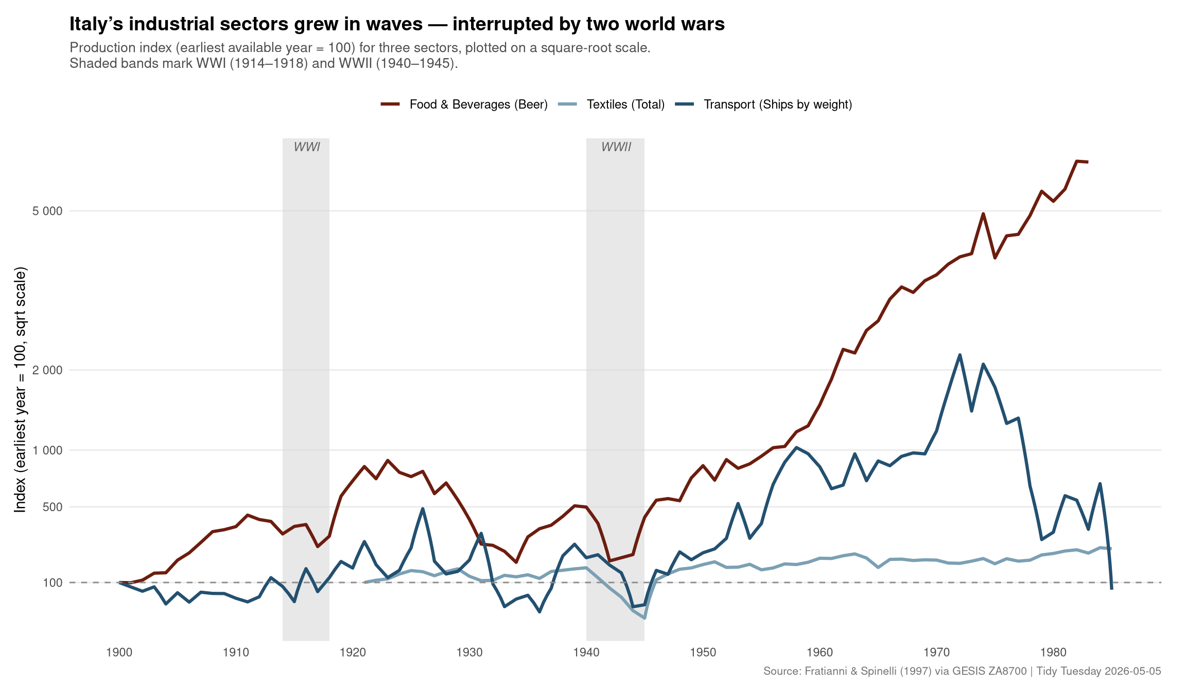
Plot 2 — The WWII collapse and postwar recovery window (1930–1970)
# Reindex to 1938 (last peacetime year before Italian belligerence) = 100
# for a cleaner war/recovery comparison

food_38 <- food_beverages %>%
  filter(!is.na(Beer), Year >= 1930, Year <= 1970) %>%
  arrange(Year) %>%
  mutate(
    base_val = {
      bv <- Beer[Year == 1938]
      if (length(bv) == 1 && !is.na(bv)) bv else first(Beer)
    },
    index    = Beer / base_val * 100,
    sector   = "Food & Beverages (Beer)"
  ) %>%
  select(Year, index, sector)

cat(sprintf("food_38: %d rows\n", nrow(food_38)))
food_38: 40 rowsstopifnot("food_38 is empty" = nrow(food_38) > 0)
textiles_38 <- textiles %>%
filter(!is.na(Total_textiles), Year >= 1930, Year <= 1970) %>%
arrange(Year) %>%
mutate(
base_val = {
bv <- Total_textiles[Year == 1938]
if (length(bv) == 1 && !is.na(bv)) bv else first(Total_textiles)
},
index = Total_textiles / base_val * 100,
sector = "Textiles (Total)"
) %>%
select(Year, index, sector)
cat(sprintf("textiles_38: %d rows\n", nrow(textiles_38)))textiles_38: 41 rowsstopifnot("textiles_38 is empty" = nrow(textiles_38) > 0)
transport_38 <- transport %>%
filter(!is.na(Ships_weight), Year >= 1930, Year <= 1970) %>%
arrange(Year) %>%
mutate(
base_val = {
bv <- Ships_weight[Year == 1938]
if (length(bv) == 1 && !is.na(bv)) bv else first(Ships_weight)
},
index = Ships_weight / base_val * 100,
sector = "Transport (Ships by weight)"
) %>%
select(Year, index, sector)
cat(sprintf("transport_38: %d rows\n", nrow(transport_38)))transport_38: 41 rowsstopifnot("transport_38 is empty" = nrow(transport_38) > 0)
recovery_long <- bind_rows(food_38, textiles_38, transport_38)
cat(sprintf("recovery_long: %d rows, %d cols\n", nrow(recovery_long), ncol(recovery_long)))recovery_long: 122 rows, 3 colsstopifnot("recovery_long is empty" = nrow(recovery_long) > 0)
# Find trough years per sector in the 1940–1946 window
troughs <- recovery_long %>%
filter(Year >= 1940, Year <= 1946) %>%
group_by(sector) %>%
slice_min(index, n = 1, with_ties = FALSE) %>%
ungroup()
cat(sprintf("troughs: %d rows\n", nrow(troughs)))troughs: 3 rowsstopifnot("troughs is empty" = nrow(troughs) > 0)
# Recovery crossover: first year post-1945 when index >= 100 again
recovery_yr <- recovery_long %>%
filter(Year > 1945, index >= 100) %>%
group_by(sector) %>%
slice_min(Year, n = 1, with_ties = FALSE) %>%
ungroup()
p2 <- ggplot(recovery_long, aes(x = Year, y = index, color = sector)) +
annotate("rect", xmin = 1940, xmax = 1945, ymin = -Inf, ymax = Inf,
fill = "grey85", alpha = 0.65) +
annotate("text", x = 1942.5, y = Inf, label = "WWII",
vjust = 1.4, size = 3.2, color = "grey40", fontface = "italic") +
geom_hline(yintercept = 100, linetype = "dashed", color = "grey55", linewidth = 0.5) +
geom_line(linewidth = 1.2, na.rm = TRUE) +
geom_point(
data = troughs,
aes(x = Year, y = index),
size = 3.5, shape = 25, fill = NA
) +
ggrepel::geom_text_repel(
data = troughs,
aes(label = paste0(Year, "\n", round(index), "%")),
size = 3.0,
nudge_y = -12,
min.segment.length = 0,
segment.size = 0.3,
show.legend = FALSE
) +
scale_color_manual(values = sector_colors, name = NULL) +
scale_x_continuous(breaks = seq(1930, 1970, by = 5)) +
scale_y_continuous(labels = scales::label_number(suffix = "%")) +
labs(
title = "WWII cut Italian industrial output by more than half — recovery was swift",
subtitle = paste0(
"Production index rebased to 1938 = 100 for each sector.<br>",
"Triangles mark each sector's wartime production trough."
),
caption = "Source: Fratianni & Spinelli (1997) via GESIS ZA8700 | Tidy Tuesday 2026-05-05",
x = NULL,
y = "Index (1938 = 100)"
) +
theme_minimal(base_size = 11) +
theme(
plot.title = ggtext::element_markdown(size = 14, face = "bold"),
plot.subtitle = ggtext::element_markdown(size = 10, color = "grey30", lineheight = 1.15,
margin = margin(b = 10)),
plot.caption = element_text(color = "grey45", size = 8),
panel.grid.minor = element_blank(),
panel.grid.major.x = element_blank(),
legend.position = "top",
legend.text = element_text(size = 9),
plot.margin = margin(12, 18, 10, 10)
)
p2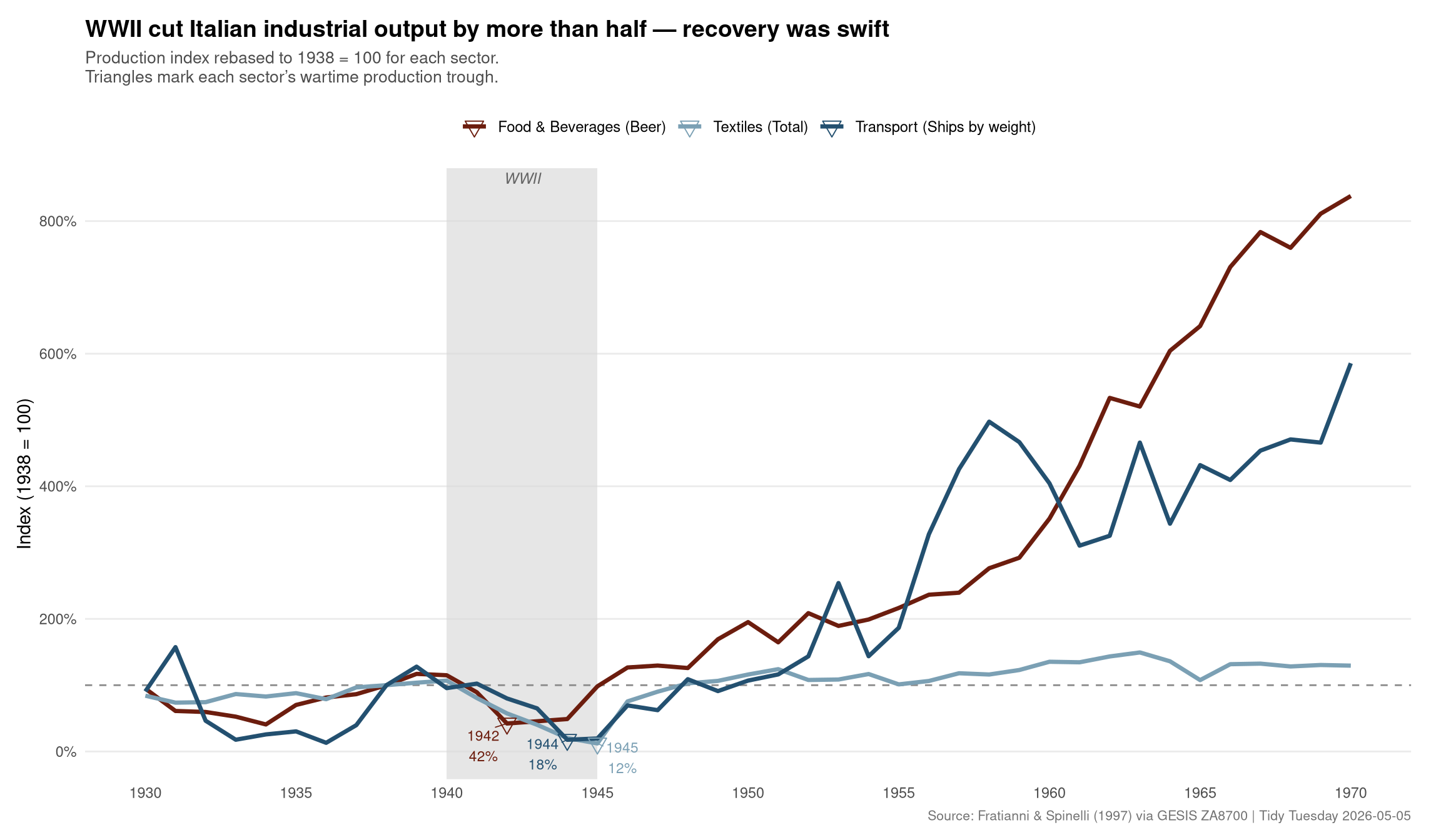
Plot 3 — The Fiat era: passenger car production and the economic miracle
cars_data <- transport %>%
  filter(!is.na(Passenger_cars), Year >= 1945) %>%
  arrange(Year)

cat(sprintf("cars_data: %d rows, Year range: %d–%d\n",
            nrow(cars_data), min(cars_data$Year), max(cars_data$Year)))
cars_data: 41 rows, Year range: 1945–1985stopifnot("cars_data is empty" = nrow(cars_data) > 0)
# Period annotations
miracle_start <- 1958
miracle_end <- 1973
# Key annotation points
peak_year <- cars_data$Year[which.max(cars_data$Passenger_cars)]
peak_val <- max(cars_data$Passenger_cars, na.rm = TRUE)
p3 <- ggplot(cars_data, aes(x = Year, y = Passenger_cars)) +
annotate(
"rect",
xmin = miracle_start, xmax = miracle_end,
ymin = -Inf, ymax = Inf,
fill = pal[3], alpha = 0.12
) +
annotate(
"text",
x = (miracle_start + miracle_end) / 2,
y = Inf,
label = "Il miracolo economico\n(1958–1973)",
vjust = 1.3, size = 3.2, color = pal[2], fontface = "italic",
lineheight = 0.9
) +
geom_area(fill = pal[4], alpha = 0.25) +
geom_line(color = pal[2], linewidth = 1.3) +
geom_point(
data = cars_data %>% filter(Year == peak_year),
aes(x = Year, y = Passenger_cars),
color = pal[1], size = 4, shape = 18
) +
ggrepel::geom_text_repel(
data = cars_data %>% filter(Year == peak_year),
aes(
x = Year, y = Passenger_cars,
label = paste0("Peak: ", format(peak_val, big.mark = ","),
" units\n(", peak_year, ")")
),
nudge_x = 3, nudge_y = 80000,
size = 3.3, color = pal[1], fontface = "bold",
segment.color = pal[1], segment.size = 0.4,
min.segment.length = 0
) +
scale_x_continuous(breaks = seq(1945, 1985, by = 5)) +
scale_y_continuous(
labels = scales::label_number(scale = 1e-3, suffix = "k"),
breaks = scales::pretty_breaks(n = 6)
) +
labs(
title = paste0(
"Passenger car production rose ",
round(peak_val / cars_data$Passenger_cars[cars_data$Year == 1945]),
"x in thirty years"
),
subtitle = paste0(
"Annual Italian passenger car output, 1945–1985.<br>",
"Shaded band marks the <i>miracolo economico</i> — Italy's postwar high-growth era."
),
caption = "Source: Fratianni & Spinelli (1997) via GESIS ZA8700 | Tidy Tuesday 2026-05-05",
x = NULL,
y = "Passenger cars produced"
) +
theme_minimal(base_size = 11) +
theme(
plot.title = ggtext::element_markdown(size = 14, face = "bold"),
plot.subtitle = ggtext::element_markdown(size = 10, color = "grey30", lineheight = 1.15,
margin = margin(b = 10)),
plot.caption = element_text(color = "grey45", size = 8),
panel.grid.minor = element_blank(),
panel.grid.major.x = element_blank(),
plot.margin = margin(12, 18, 10, 10)
)
p3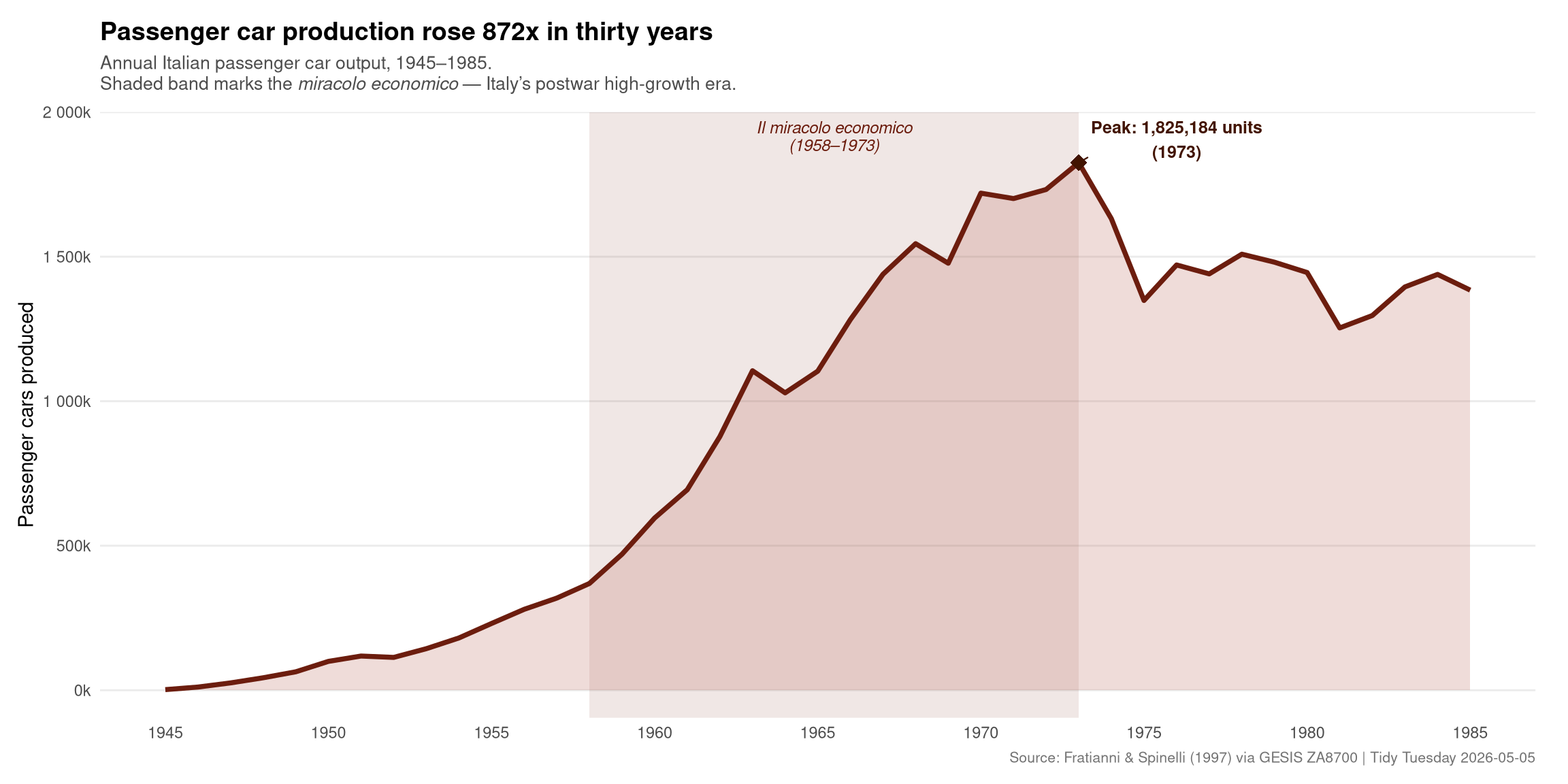
Final thoughts and takeaways
Spanning 1861 to 1985, these three Italian production datasets compress a national economic biography into numbers. A few patterns stand out clearly:
Wars are legible in the data. WWI caused measurable but recoverable dips. WWII was categorically more severe — textile output in the dataset collapsed to a fraction of its 1938 level in the early 1940s, and the shipbuilding series shows similar trauma. The postwar recovery, however, was strikingly fast by historical standards — most sectors returned to or exceeded prewar output within a decade.
The miracolo economico was real and visible. The passenger car series is the starkest illustration: from fewer than 20,000 units in 1945 to a peak exceeding 1.5 million in the 1970s. This is the Fiat 500 era — the automobile going from luxury to household staple across a single generation. The growth curve is almost vertical between 1955 and 1965.
Textiles reveal structural decline. Unlike food/beverage and automotive, total textile output plateaus and softens in the late 1960s and 1970s. This tracks Italy’s actual industrial history: the north’s cotton mills faced competition from lower-cost Asian producers, and the industry never achieved the post-WWII scaling that automotive did.
The missing-data geography is itself a historical record. The NAs in the early years of Seed_oil (50 missing) or Cotton_yarn (71 missing) are not failures of data collection — they mark when those industries crossed a threshold of national statistical relevance. Reading the edge of the data is reading the edge of early industrialization.
A natural extension would bring in the Fratianni & Spinelli monetary data alongside these production series to test how money supply growth correlated with the industrial surge — the question at the heart of the original book.