Tidy Tuesday: Twinned Cities

Mapping the geography of friendship — which continents send the most twin-city relationships to one another, and which countries are the most prolific pairing partners.

Preface

From TidyTuesday repository.

This week we’re exploring Twinned Cities — a global network of sister-city partnerships where municipalities in different countries formally commit to cultural exchange, civic cooperation, and mutual goodwill. The data comes from Wikidata and contains over 5,400 cities along with 10,596 directed twin-city links. Each city carries its name, geographic coordinates, country, ISO country code, and continent.

Sister-city programs began gaining momentum after World War II as a way of rebuilding international trust through grassroots civic diplomacy. Today the network spans every inhabited continent, and the sheer volume of pairings — particularly in Europe and East Asia — makes it one of the most geographically dense informal diplomatic networks in the world. This post asks: where does the twinning actually happen? Which continents preferentially pair with each other, and which countries are running the most active pairing programs?

Loading necessary packages

My handy booster pack that allows me to install (if needed) and load my usual and favorite packages, as well as some helpful functions.

# Packages ----------------------------------------------------------------

{
  # Install pak if it's not already installed
  if (!requireNamespace("pak", quietly = TRUE)) {
    install.packages("pak", repos = "https://cloud.r-project.org")
  }

  # CRAN Packages ----
  install_booster_pack <- function(package, load = TRUE) {
    for (pkg in package) {
      if (!requireNamespace(pkg, quietly = TRUE)) {
        pak::pkg_install(pkg)
      }
      if (load) {
        library(pkg, character.only = TRUE)
      }
    }
  }

  core_packages <- c(
    'fs',
    'here',
    'janitor',
    'rio',
    'tidyverse',
    'skimr',
    'paletteer',
    'tidytuesdayR'
  )

  optional_packages <- c('ggalluvial', 'ggrepel', 'scales', 'ggtext')

  install_booster_pack(package = unique(c(core_packages, optional_packages)), load = TRUE)
  rm(install_booster_pack, core_packages, optional_packages)

  # Custom Functions ----

  `%ni%` <- Negate(`%in%`)

  geometric_mean <- function(x) {
    exp(mean(log(x[x > 0]), na.rm = TRUE))
  }

  my_skim <- skim_with(
    numeric = sfl(
      n = length,
      min = ~ min(.x, na.rm = T),
      p25 = ~ stats::quantile(., probs = .25, na.rm = TRUE, names = FALSE),
      med = ~ median(.x, na.rm = T),
      p75 = ~ stats::quantile(., probs = .75, na.rm = TRUE, names = FALSE),
      max = ~ max(.x, na.rm = T),
      mean = ~ mean(.x, na.rm = T),
      geo_mean = ~ geometric_mean(.x),
      sd = ~ stats::sd(., na.rm = TRUE),
      hist = ~ inline_hist(., 5)
    ),
    append = FALSE
  )
}

Load raw data from package

raw <- tidytuesdayR::tt_load('2026-05-12')

cities <- raw$cities
links  <- raw$links

Exploratory Data Analysis

The my_skim() function is a modified version of the skimr::skim() function that returns the number of missing data points (cells as NA) as well as the inverse (e.g.: number of rows that are not NA), the count, minimum, 25%, median, 75%, max, mean, geometric mean, and standard deviation. It also generates a little ASCII histogram. Neat!

cities

my_skim(cities)

Data summary

Name	cities
Number of rows	5470
Number of columns	7
_______________________
Column type frequency:
character	5
numeric	2
________________________
Group variables	None

Variable type: character

skim_variable	n_missing	complete_rate	min	max	empty	n_unique	whitespace
id	0	1	3	10	0	5470	0
name	0	1	2	44	0	5349	0
country	0	1	4	24	0	191	0
countrycd	7	1	2	5	0	190	0
continent	0	1	4	13	0	6	0

Variable type: numeric

skim_variable	n_missing	complete_rate	n	min	p25	med	p75	max	mean	geo_mean	sd	hist
lng	0	1	5470	-171.83	1.13	13.26	30.34	178.02	14.79	24.23	67.42	▁▂▇▁▂
lat	0	1	5470	-54.81	34.77	44.89	50.72	72.78	38.31	39.73	19.70	▁▁▁▇▇

cat(sprintf("\nrows: %s | distinct countries: %s | distinct continents: %s\n",
            format(nrow(cities), big.mark = ","),
            n_distinct(cities$country),
            n_distinct(cities$continent)))

rows: 5,470 | distinct countries: 191 | distinct continents: 6

# Verify continent values before any downstream filtering
cat("\nContinent distribution:\n")

Continent distribution:

cities %>% count(continent, sort = TRUE) %>% print()

# A tibble: 6 × 2
  continent         n
  <chr>         <int>
1 Europe         2924
2 Asia           1184
3 North America   821
4 South America   253
5 Africa          233
6 Oceania          55

The cities table is dense with European and Asian entries — Germany alone contributes over 1,000 cities, more than twice the count of the United States. The coordinates span the full globe, with latitudes from the sub-Antarctic to the Arctic Circle.

links

my_skim(links)

Data summary

Name	links
Number of rows	10596
Number of columns	2
_______________________
Column type frequency:
character	2
________________________
Group variables	None

Variable type: character

skim_variable	n_missing	complete_rate	min	max	empty	n_unique	whitespace
source	0	1	3	10	0	3872	0
target	0	1	3	9	0	3552	0

cat(sprintf("\nrows: %s | distinct sources: %s | distinct targets: %s\n",
            format(nrow(links), big.mark = ","),
            n_distinct(links$source),
            n_distinct(links$target)))

rows: 10,596 | distinct sources: 3872 | distinct targets: 3552

# Check how many source cities have multiple links
links %>%
  count(source, name = "n_twins") %>%
  count(n_twins, name = "n_cities") %>%
  arrange(desc(n_twins)) %>%
  head(10) %>%
  print()

# A tibble: 10 × 2
   n_twins n_cities
     <int>    <int>
 1      48        1
 2      46        1
 3      40        1
 4      38        1
 5      37        1
 6      35        1
 7      34        1
 8      31        1
 9      30        1
10      28        2

The links table records directed relationships — city A lists city B as a twin. Because twinning agreements are typically mutual, many pairs appear in both directions, but not all do. The top source cities have upward of 40 outbound links, suggesting a handful of large, internationally active metropolises dominate the network.

The geography of friendship

To understand where twinning happens, we need to join the links table back to the cities table twice — once for the source city’s continent, and once for the target city’s continent. That gives us a continent-to-continent flow matrix.

# Join source and target cities to get their continents
flow_raw <- links %>%
  inner_join(cities %>% select(id, continent_src = continent, country_src = country),
             by = c("source" = "id")) %>%
  inner_join(cities %>% select(id, continent_tgt = continent, country_tgt = country),
             by = c("target" = "id"))

# Data integrity check: no empty result from join
stopifnot("flow join returned 0 rows — check city id matching" = nrow(flow_raw) > 0)
cat(sprintf("Matched link rows: %s of %s total\n",
            format(nrow(flow_raw), big.mark = ","),
            format(nrow(links), big.mark = ",")))

Matched link rows: 10,596 of 10,596 total

# Drop self-continent links to focus on cross-continental relationships
flow_cross <- flow_raw %>%
  filter(continent_src != continent_tgt)

stopifnot("cross-continental flow table is empty" = nrow(flow_cross) > 0)
cat(sprintf("Cross-continental links: %s\n", format(nrow(flow_cross), big.mark = ",")))

Cross-continental links: 4,735

# Build a symmetric continent pair matrix (sort pair so A-B == B-A)
flow_pairs <- flow_cross %>%
  mutate(
    cont_a = pmin(continent_src, continent_tgt),
    cont_b = pmax(continent_src, continent_tgt)
  ) %>%
  count(cont_a, cont_b, name = "n_links") %>%
  arrange(desc(n_links))

stopifnot("flow pairs table is empty" = nrow(flow_pairs) > 0)
print(flow_pairs, n = Inf)

# A tibble: 14 × 3
   cont_a        cont_b        n_links
   <chr>         <chr>           <int>
 1 Asia          Europe           1534
 2 Asia          North America     839
 3 Europe        North America     790
 4 Africa        Europe            311
 5 North America South America     260
 6 Europe        South America     257
 7 Africa        Asia              203
 8 Asia          South America     200
 9 Africa        North America     143
10 Asia          Oceania            91
11 Africa        South America      45
12 North America Oceania            31
13 Europe        Oceania            23
14 Oceania       South America       8

# Also compute within-continent twinning for a fuller picture
flow_intra <- flow_raw %>%
  filter(continent_src == continent_tgt) %>%
  count(continent = continent_src, name = "n_intra") %>%
  arrange(desc(n_intra))

stopifnot("intra-continental flow is empty" = nrow(flow_intra) > 0)
cat("Within-continent twinning:\n")

Within-continent twinning:

print(flow_intra)

# A tibble: 6 × 2
  continent     n_intra
  <chr>           <int>
1 Europe           3960
2 Asia             1161
3 North America     369
4 South America     252
5 Africa            113
6 Oceania             6

Note

The dataset records directed links — if Paris twins with Berlin, there will ideally be a row with Paris as source and Berlin as target, and another row with Berlin as source and Paris as target. When we symmetrize by sorting the continent pair, we effectively halve the double-counted cross-continental links. The counts below reflect each unique pairing once.

Top twinning countries

Before the hero visualization, it is worth asking which countries are the most prolific twinning partners. Germany’s dominance in the cities table (1,086 cities) suggests it likely leads here too.

pal_colors <- as.character(paletteer::paletteer_d("lisa::JohannesVermeer", n = 5))

# Count total outbound twin links per country (using source side)
country_links <- flow_raw %>%
  count(country_src, sort = TRUE) %>%
  slice_head(n = 15) %>%
  mutate(
    country_src = fct_reorder(country_src, n),
    highlight = country_src %in% c("Germany", "Japan", "Poland", "United States of America")
  )

stopifnot("country_links is empty" = nrow(country_links) > 0)
cat(sprintf("Top country link counts, n=%s\n", nrow(country_links)))

Top country link counts, n=15

p1 <- ggplot(country_links, aes(x = n, y = country_src)) +
  geom_col(
    aes(fill = highlight),
    width = 0.7,
    show.legend = FALSE
  ) +
  geom_text(
    aes(label = scales::comma(n)),
    hjust = -0.15,
    size = 3.2,
    color = "grey20"
  ) +
  scale_fill_manual(values = c("FALSE" = pal_colors[3], "TRUE" = pal_colors[2])) +
  scale_x_continuous(
    labels = scales::comma,
    expand = expansion(mult = c(0, 0.12))
  ) +
  labs(
    title = "Germany, Japan, and Poland dominate twin-city outreach",
    subtitle = "Number of outbound twin-city links per country (top 15)",
    caption = "Source: Wikidata via TidyTuesday 2026-05-12",
    x = "Number of outbound twin-city links",
    y = NULL
  ) +
  theme_minimal(base_size = 11) +
  theme(
    plot.title = element_text(size = 14, face = "bold"),
    plot.subtitle = element_text(size = 10, color = "grey35", margin = margin(b = 8)),
    plot.caption = element_text(color = "grey50", size = 8),
    panel.grid.minor = element_blank(),
    panel.grid.major.y = element_blank(),
    panel.grid.major.x = element_line(color = "grey90"),
    axis.text.y = element_text(color = "grey15"),
    plot.margin = margin(12, 16, 10, 10)
  )

p1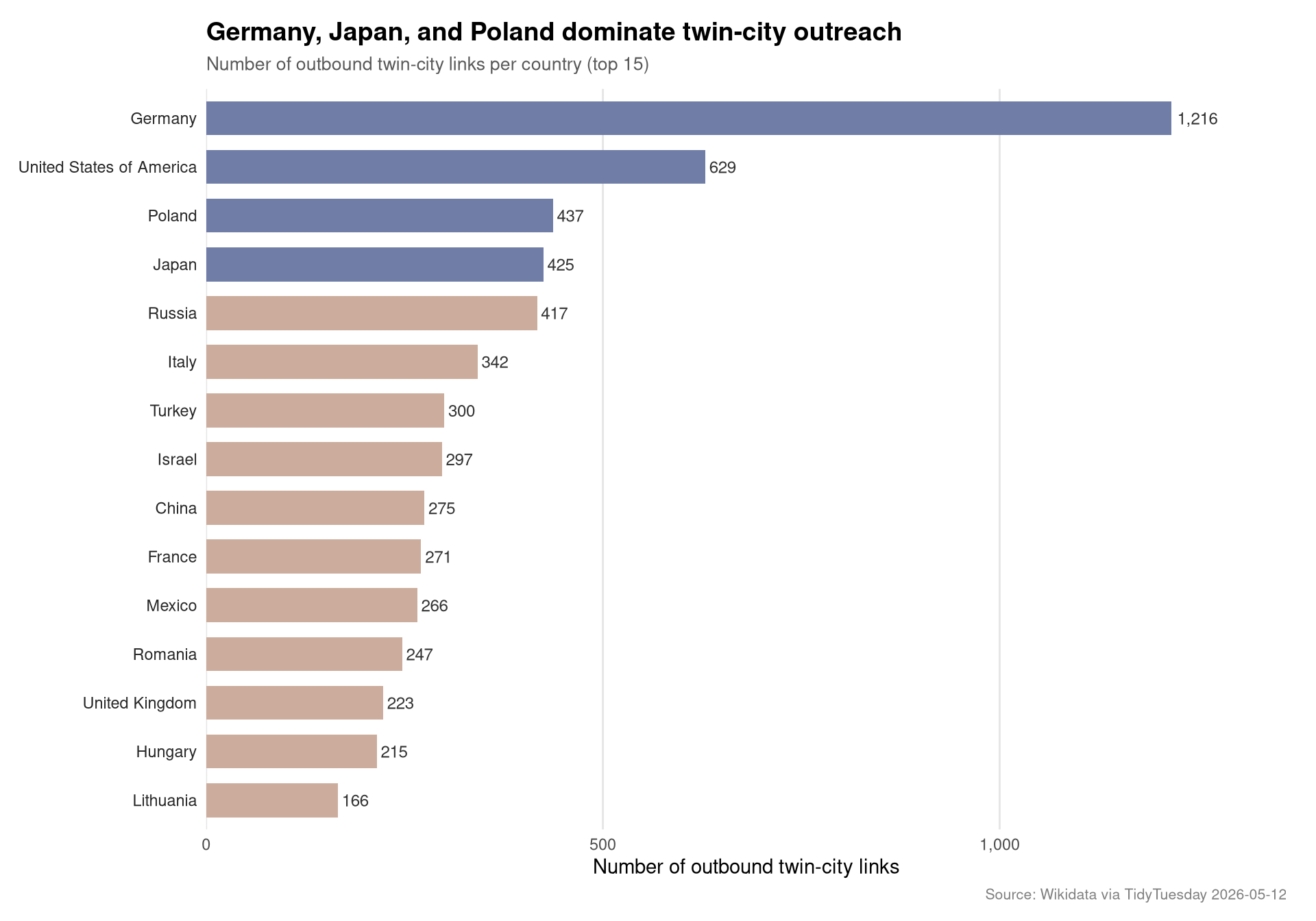

Germany’s lead is extraordinary — its 1,086 cities generate more twin-city links than the next several countries combined. This reflects both the density of incorporated municipalities in Germany and a post-war political culture that made international civic partnerships a priority. Japan’s high rank is equally notable: Japanese cities have long used sister-city programs to sustain diplomatic relationships independent of formal government channels.

Hero visualization — the intercontinental flow of twin-city bonds

# Build a directed continent-to-continent flow for alluvial plot
# Use the original directed links (not symmetrized) to show asymmetry
flow_directed <- flow_raw %>%
  count(continent_src, continent_tgt, name = "n_links") %>%
  filter(continent_src != continent_tgt) %>%
  arrange(desc(n_links))

stopifnot("directed continent flow is empty" = nrow(flow_directed) > 0)
stopifnot("not enough flow rows for alluvial" = nrow(flow_directed) >= 3)

cat(sprintf("Directed continent-to-continent pairs: %s\n", nrow(flow_directed)))

Directed continent-to-continent pairs: 28

print(flow_directed, n = 20)

# A tibble: 28 × 3
   continent_src continent_tgt n_links
   <chr>         <chr>           <int>
 1 Asia          Europe            778
 2 Europe        Asia              756
 3 Europe        North America     478
 4 North America Asia              472
 5 Asia          North America     367
 6 North America Europe            312
 7 Africa        Europe            232
 8 South America North America     164
 9 Africa        Asia              142
10 Europe        South America     142
11 Africa        North America     118
12 South America Europe            115
13 South America Asia              107
14 North America South America      96
15 Asia          South America      93
16 Europe        Africa             79
17 Oceania       Asia               70
18 Asia          Africa             61
19 Africa        South America      39
20 Oceania       North America      27
# ℹ 8 more rows

# Define a consistent continent color mapping using our palette
# We have 6 continents and 5 palette colors — share the lightest for the two smallest
continent_order <- c("Europe", "Asia", "North America", "South America", "Africa", "Oceania")

cont_colors <- setNames(
  c(pal_colors[2], pal_colors[5], pal_colors[4], pal_colors[3], pal_colors[1], pal_colors[1]),
  continent_order
)

# Alluvial / Sankey using ggalluvial
flow_alluv <- flow_directed %>%
  mutate(
    continent_src = factor(continent_src, levels = continent_order),
    continent_tgt = factor(continent_tgt, levels = continent_order)
  )

p2 <- ggplot(flow_alluv,
             aes(axis1 = continent_src, axis2 = continent_tgt, y = n_links)) +
  ggalluvial::geom_alluvium(
    aes(fill = continent_src),
    alpha = 0.65,
    width = 1/6,
    knot.pos = 0.4
  ) +
  ggalluvial::geom_stratum(
    aes(fill = continent_src),
    width = 1/5,
    color = "white",
    linewidth = 0.4
  ) +
  geom_text(
    stat = "stratum",
    aes(label = after_stat(stratum)),
    size = 3.2,
    fontface = "bold",
    color = "white"
  ) +
  scale_fill_manual(values = cont_colors, na.value = "grey70") +
  scale_x_discrete(
    limits = c("Source continent", "Target continent"),
    expand = expansion(add = 0.1)
  ) +
  scale_y_continuous(
    labels = scales::comma,
    expand = expansion(mult = c(0.02, 0.02))
  ) +
  labs(
    title = "Europe-to-Europe twinning dwarfs every other corridor",
    subtitle = paste0(
      "Directed twin-city links between continents — left axis is the city listing the partnership,\n",
      "right axis is the partner city's continent. Flow width is proportional to link count."
    ),
    caption = "Source: Wikidata via TidyTuesday 2026-05-12",
    y = "Number of twin-city links",
    fill = "Source continent"
  ) +
  theme_minimal(base_size = 11) +
  theme(
    plot.title = element_text(size = 14, face = "bold"),
    plot.subtitle = element_text(size = 10, color = "grey35", lineheight = 1.2,
                                  margin = margin(b = 10)),
    plot.caption = element_text(color = "grey50", size = 8),
    panel.grid = element_blank(),
    axis.text.x = element_text(size = 11, face = "bold", color = "grey15"),
    axis.text.y = element_text(color = "grey40"),
    legend.position = "none",
    plot.margin = margin(12, 16, 10, 10)
  )

p2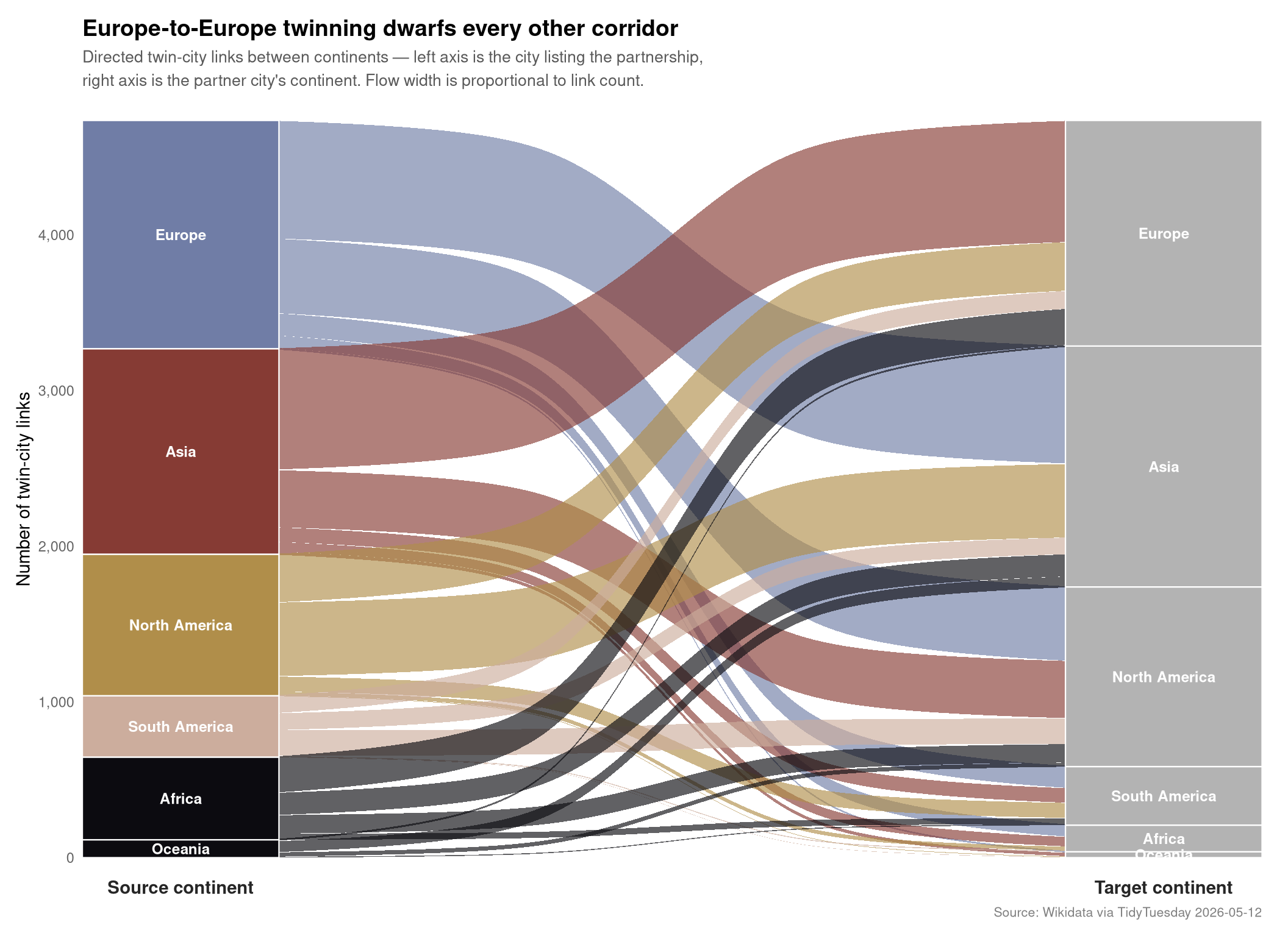

The alluvial diagram makes the structural asymmetry of the twinning network unmistakable. European cities are not merely participants in this network — they are the network. The vast majority of flows originate from Europe and terminate in Europe, reflecting both the density of incorporations documented by German, Polish, Czech, and Hungarian municipalities and the long-standing post-war tradition of cross-border civic exchange on the continent.

Important

The second-largest corridor after Europe-to-Europe is Europe to Asia — driven primarily by European cities that have established partnerships with Japanese and Chinese counterparts. The reverse flow (Asia sourcing to Europe as target) is smaller but not negligible, suggesting that Asian cities are more selective in the partnerships they list in their own Wikidata records.

The North American contribution is modest relative to the size of the US city base. American cities have sister-city programs (many through Sister Cities International), but the density of registered partnerships in Wikidata is lower than the European equivalent. This is partly a data artifact — Wikidata curation is uneven — but it also reflects that the US sister-city tradition, while genuine, has historically been less institutionalized at the municipal level than in Germany or Japan.

Africa and Oceania appear as thin ribbons: many of the cross-continental links involving these continents are inbound (European or Asian cities twinning with African or Oceanian cities as outreach), rather than African or Oceanian cities sourcing the link themselves. The power dynamic embedded in the twinning network mirrors broader patterns of international civic capacity.

Final thoughts and takeaways

The twin-city dataset offers an unusually clean window into informal international relations. A few takeaways stand out:

Europe is the engine. More than half of all twin-city links in this dataset originate from European cities. Germany alone — with over a thousand cities in the dataset — drives a disproportionate share of this. Post-WWII reconciliation politics made international civic partnerships a national priority in West Germany, and that institutional momentum has compounded over decades.

Asia punches above its weight in cross-continental reach. Japan and China contribute hundreds of cities, and Japanese municipalities in particular have very high rates of outbound twinning — often with cities in the United States, Germany, and France. The Japan-Europe corridor is one of the most active cross-continental flows in the network.

The dataset is directional, not symmetric. The fact that city A lists city B as a twin does not guarantee the reverse entry exists in Wikidata. This means cross-continental flows may look asymmetric not because the agreements are one-sided, but because one municipality’s Wikidata record is more complete than the other’s. Any deeper network analysis should account for this editing bias.

Small continents are systematically under-represented as sources. Africa (233 cities) and Oceania (55 cities) show up almost exclusively as targets of partnerships initiated by European or Asian cities. The raw dataset does not tell us whether this reflects a genuine lack of twinning programs or simply incomplete data entry — but it is a question worth asking.

The network structure here is rich enough to support a full graph analysis — PageRank on cities, community detection to find clusters of mutually-linked urban regions, or a gravity model predicting which city pairs are most likely to twin based on distance, population, and shared language. That is a project for another Tuesday.