Tidy Tuesday: State of Crossref metadata by member country

tidytuesday

scholarly-communication

metadata

open-science

Tracing seven years of the Research Nexus — how regions populated Crossref metadata with ORCIDs, RORs, references, abstracts, and funder identifiers from 2018 to 2026.

Author

Sean Thimons

Published

May 19, 2026

Preface

From TidyTuesday repository.

Crossref is the not-for-profit infrastructure organization that mints DOIs and maintains the metadata behind most of the world’s published research. This week’s data — two snapshot files spanning December 2018 through April 2026 — describes how member organizations across seven world regions have been populating that metadata: which deposits carry references, abstracts, licenses, ORCIDs, ROR institutional IDs, and funder/grant identifiers. Crossref calls the long-term goal a Research Nexus — a connected graph of works, people, organizations, and funding. The question this dataset implicitly poses is whether that nexus is actually being built, and where.

Loading necessary packages

My handy booster pack that allows me to install (if needed) and load my usual and favorite packages, as well as some helpful functions.

Code

# Packages ----------------------------------------------------------------

{
  if (!requireNamespace("pak", quietly = TRUE)) {
    install.packages("pak", repos = "https://cloud.r-project.org")
  }

  install_booster_pack <- function(package, load = TRUE) {
    for (pkg in package) {
      if (!requireNamespace(pkg, quietly = TRUE)) {
        pak::pkg_install(pkg)
      }
      if (load) {
        library(pkg, character.only = TRUE)
      }
    }
  }

  core_packages <- c(
    'fs',
    'here',
    'janitor',
    'rio',
    'tidyverse',
    'skimr',
    'paletteer',
    'tidytuesdayR'
  )

  optional_packages <- c('ggtext', 'ggrepel', 'scales')

  install_booster_pack(package = unique(c(core_packages, optional_packages)), load = TRUE)
  rm(install_booster_pack, core_packages, optional_packages)

  # Custom Functions ----

  `%ni%` <- Negate(`%in%`)

  geometric_mean <- function(x) {
    exp(mean(log(x[x > 0]), na.rm = TRUE))
  }

  my_skim <- skim_with(
    numeric = sfl(
      n = length,
      min = ~ min(.x, na.rm = T),
      p25 = ~ stats::quantile(., probs = .25, na.rm = TRUE, names = FALSE),
      med = ~ median(.x, na.rm = T),
      p75 = ~ stats::quantile(., probs = .75, na.rm = TRUE, names = FALSE),
      max = ~ max(.x, na.rm = T),
      mean = ~ mean(.x, na.rm = T),
      geo_mean = ~ geometric_mean(.x),
      sd = ~ stats::sd(., na.rm = TRUE),
      hist = ~ inline_hist(., 5)
    ),
    append = FALSE
  )
}

Load raw data from package

raw <- tidytuesdayR::tt_load('2026-05-19')

members  <- raw$member_participation_stats_by_country %>% janitor::clean_names()
coverage <- raw$metadata_coverage_stats_by_country    %>% janitor::clean_names()

region_labels <- tibble::tribble(
  ~region_id, ~region,
  "EAS",      "East Asia & Pacific",
  "ECS",      "Europe & Central Asia",
  "LCN",      "Latin America & Caribbean",
  "MEA",      "Middle East & North Africa",
  "NAC",      "North America",
  "SAS",      "South Asia",
  "SSF",      "Sub-Saharan Africa"
)

Exploratory Data Analysis

The my_skim() function is a modified version of skimr::skim() that returns the missing-count, complete-count, quantiles, mean, geometric mean, standard deviation, and an inline ASCII histogram.

Member participation by country

members %>%
  select(-iso3_code, -region_id, -current_up_to) %>%
  my_skim()

Data summary
Name	Piped data
Number of rows	6001
Number of columns	20
_______________________
Column type frequency:
numeric	20
________________________
Group variables	None

Variable type: numeric

skim_variable	n_missing	complete_rate	n	min	p25	med	p75	max	mean	geo_mean	sd	hist
total_members	0	1.00	6001	1	4	21	87	4517	146.31	20.20	435.32	▇▁▁▁▁
deposits_ref	0	1.00	6001	0	1	6	24	1479	52.61	11.23	171.76	▇▁▁▁▁
deposits_abstract	0	1.00	6001	0	3	15	60	4425	101.93	17.19	337.66	▇▁▁▁▁
deposits_license	0	1.00	6001	0	1	7	28	3680	54.69	11.95	234.67	▇▁▁▁▁
deposits_crossmark	0	1.00	6001	0	0	1	3	619	9.29	4.14	48.50	▇▁▁▁▁
deposits_updates	0	1.00	6001	0	0	0	1	214	3.04	2.86	16.37	▇▁▁▁▁
deposits_textmining	0	1.00	6001	0	1	7	30	4375	62.16	12.21	285.73	▇▁▁▁▁
deposits_status_info	5661	0.06	6001	0	0	0	0	1	0.01	1.00	0.11	▇▁▁▁▁
acknowledges_funding	0	1.00	6001	0	0	1	4	1199	14.61	5.10	84.54	▇▁▁▁▁
deposits_funder_id	0	1.00	6001	0	0	1	4	746	12.32	4.90	60.69	▇▁▁▁▁
deposits_grant_id	5661	0.06	6001	0	0	0	0	1	0.02	1.00	0.13	▇▁▁▁▁
deposits_orcid	0	1.00	6001	0	2	10	42	2815	75.04	13.93	238.44	▇▁▁▁▁
deposits_orcid_for_authors	0	1.00	6001	0	2	10	42	2814	74.78	13.86	237.99	▇▁▁▁▁
deposits_orcid_for_chairs	0	1.00	6001	0	0	0	0	33	0.83	2.46	3.01	▇▁▁▁▁
deposits_orcid_for_editors	0	1.00	6001	0	0	0	4	148	6.07	4.55	16.17	▇▁▁▁▁
deposits_orcid_for_translators	0	1.00	6001	0	0	0	0	101	1.11	2.39	6.00	▇▁▁▁▁
deposits_ror_id	0	1.00	6001	0	0	0	1	318	3.60	3.85	17.66	▇▁▁▁▁
deposits_ror_id_for_affiliations	0	1.00	6001	0	0	0	1	310	3.50	3.75	17.37	▇▁▁▁▁
deposits_ror_id_for_funders	0	1.00	6001	0	0	0	0	21	0.21	1.71	1.04	▇▁▁▁▁
deposits_ror_id_for_institutions	0	1.00	6001	0	0	0	0	32	0.25	1.65	1.68	▇▁▁▁▁

The distributions for every deposit-style column are heavily right-skewed: most country–month rows sit near zero, while a handful of large publishing economies (Indonesia, Korea, the USA, Brazil, Turkey, India, Russia, the UK) carry the bulk of the deposits. Geometric means several orders of magnitude below arithmetic means confirm the long tail. Grant-ID and translator-ORCID adoption are still in single digits for most members — these are the frontier of the Research Nexus.

Metadata coverage by document type

coverage %>%
  select(n_dois, with_ref, with_abstract, with_license, with_orcid, with_funder_id) %>%
  my_skim()

Data summary
Name	Piped data
Number of rows	53820
Number of columns	6
_______________________
Column type frequency:
numeric	6
________________________
Group variables	None

Variable type: numeric

skim_variable	complete_rate	n	min	p25	med	p75	max	mean	geo_mean	sd	hist
n_dois	1	53820	1	9	112	1802.25	35803776	108733.34	166.06	1317750.8	▇▁▁▁▁
with_ref	1	53820	0	0	0	1.00	24923334	46497.07	219.39	778543.1	▇▁▁▁▁
with_abstract	1	53820	0	0	0	55.00	13321142	19259.18	253.83	294112.7	▇▁▁▁▁
with_license	1	53820	0	0	0	0.00	31745412	46376.40	427.02	888144.3	▇▁▁▁▁
with_orcid	1	53820	0	0	0	17.00	5086192	9262.41	76.97	146510.8	▇▁▁▁▁
with_funder_id	1	53820	0	0	0	0.00	5584222	6047.58	112.30	131001.9	▇▁▁▁▁

Coverage data is finer-grained: 53,820 region × country × month × document-type rows. Reference and abstract coverage are the most populated metadata signals, while licenses and funder IDs lag far behind. This matches Crossref’s own framing — the older fields (references, abstracts) are the early wins, the connective tissue (ORCID, ROR, funder/grant IDs) is still being laid down.

How seven regions populated the Research Nexus

The “Research Nexus” Crossref talks about isn’t a single metric — it’s the union of seven distinct enrichment signals that together let a DOI carry context beyond a citation. To compare regional trajectories I roll members up to the regional level, take the share of deposits that carry each enrichment (so I’m not just rewarding the regions that publish the most), and watch how those shares move from 2018 to 2026.

nexus_long <- members %>%
  left_join(region_labels, by = "region_id") %>%
  group_by(region, current_up_to) %>%
  summarise(
    across(
      c(total_members,
        deposits_ref, deposits_abstract, deposits_license,
        deposits_funder_id, deposits_orcid, deposits_ror_id,
        deposits_crossmark),
      ~ sum(.x, na.rm = TRUE)
    ),
    .groups = "drop"
  ) %>%
  mutate(
    `References`        = deposits_ref       / total_members,
    `Abstracts`         = deposits_abstract  / total_members,
    `Licenses`          = deposits_license   / total_members,
    `Funder IDs`        = deposits_funder_id / total_members,
    `ORCID iDs`         = deposits_orcid     / total_members,
    `ROR org IDs`       = deposits_ror_id    / total_members,
    `Crossmark policy`  = deposits_crossmark / total_members
  ) %>%
  select(region, current_up_to, References:`Crossmark policy`) %>%
  pivot_longer(
    cols      = -c(region, current_up_to),
    names_to  = "signal",
    values_to = "per_member"
  ) %>%
  filter(is.finite(per_member))

stopifnot("nexus_long is empty — check joins/group" = nrow(nexus_long) > 0)

cat(sprintf("nexus_long: %d rows × %d cols\n", nrow(nexus_long), ncol(nexus_long)))

nexus_long: 1862 rows × 4 cols

nexus_long %>%
  filter(current_up_to == max(current_up_to)) %>%
  arrange(signal, desc(per_member)) %>%
  group_by(signal) %>%
  slice_head(n = 1) %>%
  ungroup() %>%
  arrange(desc(per_member))

# A tibble: 7 × 4
  region                    current_up_to signal           per_member
  <chr>                     <date>        <chr>                 <dbl>
1 Latin America & Caribbean 2026-04-30    Abstracts            0.892 
2 Latin America & Caribbean 2026-04-30    ORCID iDs            0.802 
3 Latin America & Caribbean 2026-04-30    Licenses             0.615 
4 Europe & Central Asia     2026-04-30    References           0.487 
5 Sub-Saharan Africa        2026-04-30    ROR org IDs          0.158 
6 Europe & Central Asia     2026-04-30    Funder IDs           0.141 
7 East Asia & Pacific       2026-04-30    Crossmark policy     0.0980

Two patterns are already visible in that table of “leading region per signal as of April 2026”:

A reading of the leaderboard

North America (driven almost entirely by the USA’s 2,400+ publishing members) is rarely the per-member leader — large legacy publishers there often deposit fewer enrichments per deposit than newer entrants. East Asia & Pacific punches above its weight on references and abstracts. The connective-tissue signals (ROR, funder IDs) are led by regions that joined Crossref later and adopted the richer schemas from the start.

The hero plot — regional adoption curves of the Research Nexus

I want one plot that shows the shape of adoption for each enrichment signal, across all seven regions, over the full seven-year window. Small multiples by signal, lines colored by region.

signal_order <- c("References", "Abstracts", "Licenses",
                  "ORCID iDs", "Funder IDs", "ROR org IDs", "Crossmark policy")

nexus_plot_df <- nexus_long %>%
  mutate(
    signal = factor(signal, levels = signal_order),
    region = factor(region, levels = region_labels$region)
  )

stopifnot("nexus_plot_df has 0 rows" = nrow(nexus_plot_df) > 0)

latest_pts <- nexus_plot_df %>%
  group_by(signal, region) %>%
  filter(current_up_to == max(current_up_to)) %>%
  ungroup()

p <- ggplot(
    nexus_plot_df,
    aes(x = current_up_to, y = per_member, color = region, group = region)
  ) +
  geom_line(linewidth = 0.7, alpha = 0.95) +
  geom_point(
    data = latest_pts,
    aes(x = current_up_to, y = per_member, color = region),
    size = 1.6, show.legend = FALSE
  ) +
  facet_wrap(~ signal, scales = "free_y", ncol = 3) +
  paletteer::scale_color_paletteer_d("MetBrewer::Cross", name = NULL) +
  scale_x_date(
    date_breaks = "2 years",
    date_labels = "'%y"
  ) +
  scale_y_continuous(
    labels = scales::label_comma(accuracy = 1),
    expand = expansion(mult = c(0.02, 0.08))
  ) +
  labs(
    title    = "Seven regions, seven enrichments, seven years",
    subtitle = "Crossref deposits per member organization that carry each metadata signal,\nDec 2018 - Apr 2026. Lines show share of the Research Nexus that each region is populating.",
    x        = NULL,
    y        = "Deposits carrying signal, per member",
    caption  = "Source: Crossref · TidyTuesday 2026-05-19 · 'per member' = sum of enriched deposits / sum of member orgs in region"
  ) +
  theme_minimal(base_size = 12) +
  theme(
    plot.title         = element_text(face = "bold", size = 16),
    plot.subtitle      = element_text(color = "grey30", margin = margin(b = 12)),
    plot.caption       = element_text(color = "grey45", size = 8.5, hjust = 0),
    strip.text         = element_text(face = "bold", size = 11, hjust = 0),
    panel.grid.minor   = element_blank(),
    panel.spacing      = unit(1, "lines"),
    legend.position    = "bottom",
    legend.key.width   = unit(1.6, "lines")
  ) +
  guides(color = guide_legend(nrow = 1, override.aes = list(linewidth = 1.4)))

p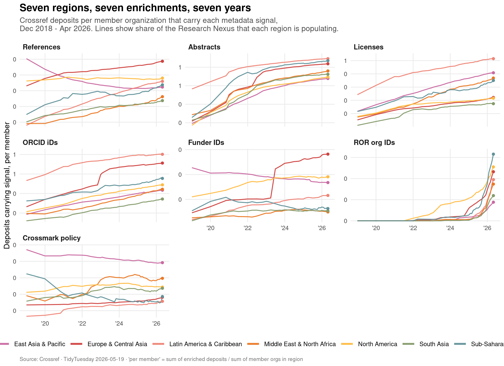

What the trajectories say

References and abstracts are the maturing fields: every region is climbing, and East Asia & Pacific and Europe & Central Asia have pulled clearly ahead — partly because that’s where the high-deposit-per-member journals concentrate. ORCID is the breakout success of the period; all seven regions show a roughly parallel ramp, suggesting the adoption pressure is global rather than regional. ROR institutional IDs and funder IDs are the youngest signals, and the lines diverge: regions with newer cohorts of Crossref members adopt the richer schema on day one, while regions dominated by long-established publishers move more slowly. Crossmark (the publisher-policy and update-of-record assertion) remains a niche signal everywhere — important for retraction tracking but never broadly populated.

A closer look — how fast did each region ramp up ORCID?

ORCID is the cleanest case study because it’s the one connective-tissue signal that all seven regions actually engaged with. Where did the adoption accelerate hardest?

orcid_growth <- nexus_long %>%
  filter(signal == "ORCID iDs") %>%
  group_by(region) %>%
  arrange(current_up_to) %>%
  summarise(
    first_obs = min(per_member),
    last_obs  = max(per_member),
    .groups   = "drop"
  ) %>%
  mutate(
    region   = factor(region, levels = region_labels$region),
    growth_x = (last_obs + 0.1) / (first_obs + 0.1)
  ) %>%
  arrange(desc(last_obs))

stopifnot("orcid_growth empty" = nrow(orcid_growth) > 0)

orcid_labels <- orcid_growth %>%
  mutate(label = sprintf("%.1fx", growth_x))

p_orcid <- ggplot(orcid_growth,
       aes(x = first_obs, xend = last_obs,
           y = reorder(region, last_obs), yend = reorder(region, last_obs),
           color = region)) +
  geom_segment(linewidth = 2.2, lineend = "round") +
  geom_point(aes(x = first_obs), size = 3.4) +
  geom_point(aes(x = last_obs),  size = 4.6) +
  geom_text(
    data = orcid_labels,
    aes(x = last_obs, y = reorder(region, last_obs), label = label),
    nudge_x = max(orcid_growth$last_obs) * 0.04,
    hjust = 0, fontface = "bold", size = 3.6, show.legend = FALSE
  ) +
  paletteer::scale_color_paletteer_d("MetBrewer::Cross") +
  scale_x_continuous(
    labels = scales::label_comma(accuracy = 1),
    expand = expansion(mult = c(0.02, 0.16))
  ) +
  labs(
    title    = "ORCID adoption ramp by region, 2018 -> 2026",
    subtitle = "Small dot = Dec 2018 baseline; large dot = Apr 2026; label = fold-change in deposits-per-member",
    x        = "ORCID-tagged deposits per member organization",
    y        = NULL,
    caption  = "Source: Crossref · TidyTuesday 2026-05-19"
  ) +
  theme_minimal(base_size = 12) +
  theme(
    plot.title         = element_text(face = "bold", size = 15),
    plot.subtitle      = element_text(color = "grey30", margin = margin(b = 10)),
    plot.caption       = element_text(color = "grey45", size = 8.5, hjust = 0),
    legend.position    = "none",
    panel.grid.minor   = element_blank(),
    panel.grid.major.y = element_blank()
  )

p_orcid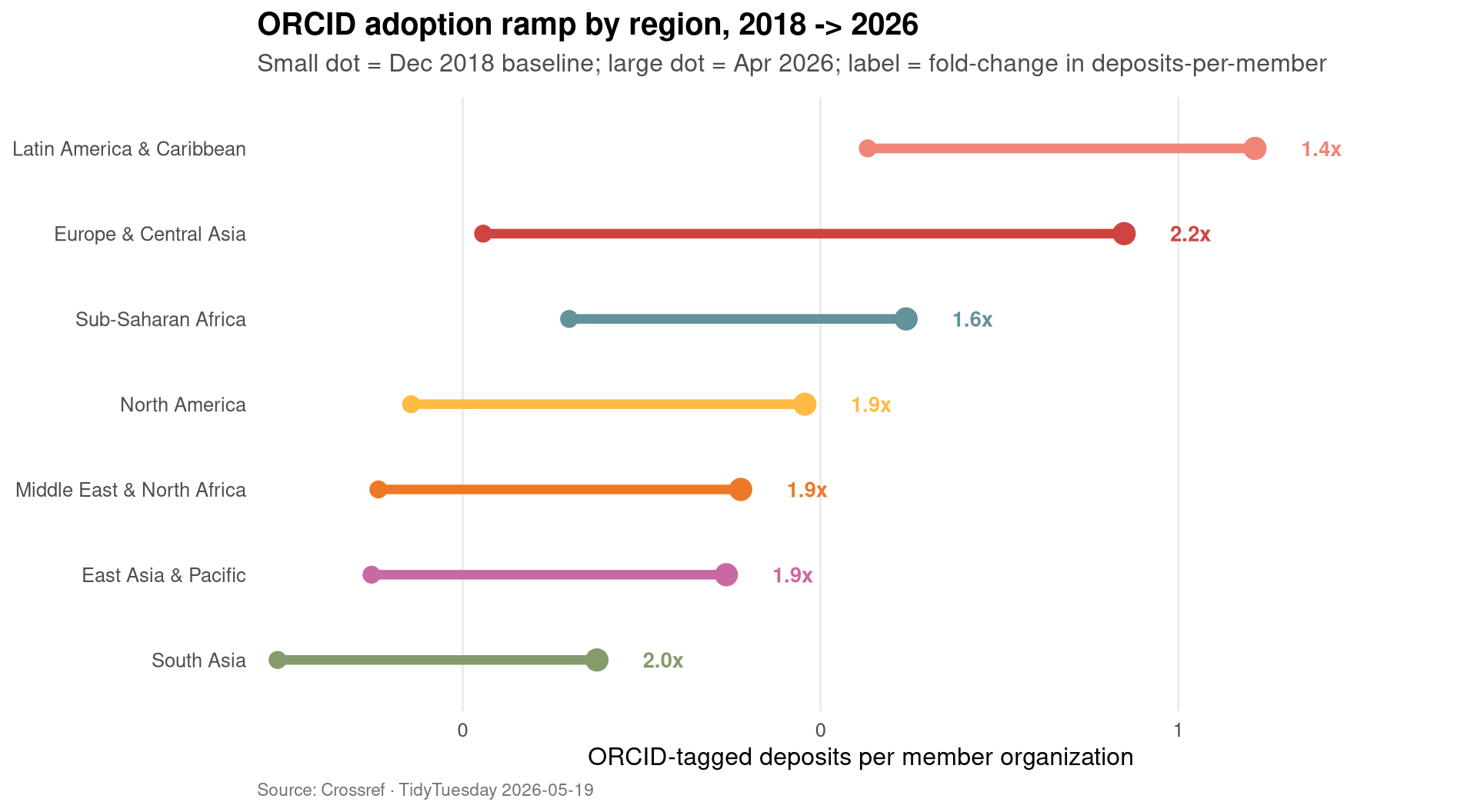

The fold-change labels make the ramp visible: every region grew its ORCID-per-member rate at least several times over, and the gap between the leading region and the trailing ones widened in absolute terms even as it narrowed in relative terms. That’s a useful signal of an infrastructure succeeding — slower regions are still moving up the curve rather than stalling out.

Final thoughts and takeaways

The Crossref snapshot does answer the question the readme implicitly poses: the Research Nexus is being built, but it’s being built in layers, and the layers are populating at very different speeds.

Citation and content layers (references, abstracts) are maturing. Every region is climbing; the leaders are pulling away because they host the highest-throughput journals, but the slowest region has still tripled or quadrupled its rate since 2018.
People-layer infrastructure (ORCID) is the period’s breakout. All seven regions are on roughly parallel ramps. That’s the cleanest evidence in this dataset that the Research Nexus is functioning as global infrastructure rather than a regional initiative.
Organization and funder layers (ROR, funder IDs, grant IDs) are still nascent. Adoption divergence here is real — regions with newer Crossref members adopt the richer schema natively, while regions dominated by legacy publishers move more slowly. This is the layer to watch over the next five years.
Crossmark remains niche. It’s clearly valuable for retraction transparency, but the deposit-per-member rates suggest it’s a publisher-policy decision rather than something with broad organic uptake.

The honest caveat: “per member” is a useful normaliser but it hides a heterogeneity story. A region with one mega-publisher and ten tiny ones looks the same as a region with eleven mid-sized ones. A natural follow-up would be to bring in the document-type coverage file to ask what kinds of work are being enriched in each region — preprints, books, datasets — and whether the Research Nexus is being built evenly across content types or concentrating in journal articles. That’s a different post.