Tidy Tuesday: European Parenting Leave Policies

tidytuesday

policy

europe

labor

Half a century of paid parental leave entitlements across 21 European countries — who treats new parents most generously, and how the policy mix has shifted from short maternity windows to long shared parental terms.

Author

Sean Thimons

Published

June 2, 2026

Preface

From TidyTuesday repository.

The European Parenting Leave Policies (EPLP) dataset captures the legal duration and design of statutory maternity, paternity, and parental leave for 21 European countries from 1970 through 2024. Each row represents one country-year, with detailed fields for leave duration (in weeks), wage replacement rates, caps, eligibility, and which parent may claim each entitlement. The data was compiled by Daniela Rohrbach-Schmidt and colleagues and reflects the policy as legislated, not actual take-up.

Loading necessary packages

My handy booster pack that allows me to install (if needed) and load my usual and favorite packages, as well as some helpful functions.

Code

{
  if (!requireNamespace("pak", quietly = TRUE)) {
    install.packages("pak", repos = "https://cloud.r-project.org")
  }

  install_booster_pack <- function(package, load = TRUE) {
    for (pkg in package) {
      if (!requireNamespace(pkg, quietly = TRUE)) {
        pak::pkg_install(pkg)
      }
      if (load) {
        library(pkg, character.only = TRUE)
      }
    }
  }

  core_packages <- c(
    'fs',
    'here',
    'janitor',
    'rio',
    'tidyverse',
    'skimr',
    'paletteer',
    'tidytuesdayR'
  )

  optional_packages <- c('ggtext', 'ggrepel', 'scales', 'MetBrewer')

  install_booster_pack(package = unique(c(core_packages, optional_packages)), load = TRUE)
  rm(install_booster_pack, core_packages, optional_packages)

  `%ni%` <- Negate(`%in%`)

  geometric_mean <- function(x) {
    exp(mean(log(x[x > 0]), na.rm = TRUE))
  }

  my_skim <- skim_with(
    numeric = sfl(
      n = length,
      min = ~ min(.x, na.rm = T),
      p25 = ~ stats::quantile(., probs = .25, na.rm = TRUE, names = FALSE),
      med = ~ median(.x, na.rm = T),
      p75 = ~ stats::quantile(., probs = .75, na.rm = TRUE, names = FALSE),
      max = ~ max(.x, na.rm = T),
      mean = ~ mean(.x, na.rm = T),
      geo_mean = ~ geometric_mean(.x),
      sd = ~ stats::sd(., na.rm = TRUE),
      hist = ~ inline_hist(., 5)
    ),
    append = FALSE
  )
}

Load raw data from package

raw <- tidytuesdayR::tt_load('2026-06-02')

eplp <- raw$eplp %>% janitor::clean_names()

Exploratory Data Analysis

The my_skim() function is a modified version of the skimr::skim() function that returns the number of missing data points (cells as NA) as well as the inverse (e.g.: number of rows that are not NA), the count, minimum, 25%, median, 75%, max, mean, geometric mean, and standard deviation. It also generates a little ASCII histogram. Neat!

EPLP

eplp %>%
  select(country, year, mat_m_ld_bb, mat_m_ld_ab, co_ld, par1_ld, par2_ld, par3_ld) %>%
  my_skim()

Data summary
Name	Piped data
Number of rows	1155
Number of columns	8
_______________________
Column type frequency:
character	1
numeric	7
________________________
Group variables	None

Variable type: character

skim_variable	n_missing	complete_rate	min	max	empty	n_unique	whitespace
country	0	1	2	2	0	21	0

Variable type: numeric

skim_variable	complete_rate	n	min	p25	med	p75	max	mean	geo_mean	sd	hist
year	1	1155	1970	1983	1997.00	2011.00	2024.00	1997.00	1996.94	15.88	▇▇▇▇▇
mat_m_ld_bb	1	1155	0	0	0.00	6.00	8.70	2.38	4.43	3.07	▇▂▁▂▂
mat_m_ld_ab	1	1155	0	0	6.00	8.00	20.00	5.00	6.33	4.54	▇▆▁▁▁
co_ld	1	1155	0	0	0.00	2.00	28.00	1.37	1.70	3.12	▇▁▁▁▁
par1_ld	1	1155	0	0	25.71	48.80	186.71	36.17	44.49	46.66	▇▂▁▁▁
par2_ld	1	1155	0	0	0.00	13.04	186.71	20.42	46.89	41.77	▇▁▁▁▁
par3_ld	1	1155	0	0	0.00	26.33	98.36	13.42	29.59	20.80	▇▂▁▁▁

cat("\nCountries (n =", length(unique(eplp$country)), "):\n")


Countries (n = 21 ):

print(sort(unique(eplp$country)))

 [1] "AT" "BE" "CZ" "DE" "DK" "EE" "ES" "FI" "FR" "GR" "HU" "IE" "IT" "LT" "NL"
[16] "NO" "PL" "SE" "SI" "SK" "UK"

cat("\nYear coverage:", min(eplp$year), "to", max(eplp$year), "\n")


Year coverage: 1970 to 2024

The frame is a balanced country-year panel: 21 countries × 55 years = 1,155 rows, with no missing country or year. Leave-duration variables (in weeks) are uniformly observed across the panel. The eligibility/cap fields are sparser — the codebook uses -98 for “not applicable” rather than NA, which would mislead a naive mean() if we used those columns directly.

The leave-duration columns split cleanly into three policy buckets:

Maternity (mat_m_ld_bb, mat_m_ld_ab) — weeks of mother-only leave before and after birth.
Co/paternity (co_ld) — short leave reserved for the second parent.
Parental (par1_ld, par2_ld, par3_ld) — successive tiers of paid parental leave that may be shared, transferred, or earmarked depending on country.

Note

The codebook draws a careful distinction between maternity (medical leave around childbirth, mother-only) and parental (child-care leave, often shareable). Many casual comparisons of “how much leave does country X offer” collapse the two; this dataset lets us keep them separate.

How generous is paid parental leave across Europe?

The headline question this dataset invites is the obvious one: in 2024, who actually offers the most paid leave, and what is it made of? A single “total weeks” number hides the policy design — a country with 40 weeks of mother-only maternity leave is doing something very different from one with 40 weeks of shareable parental leave. So the story has to be told as a decomposition, not a scalar.

leave_2024 <- eplp %>%
  filter(year == 2024) %>%
  transmute(
    country,
    Maternity     = mat_m_ld_bb + mat_m_ld_ab,
    `Co / paternity` = co_ld,
    `Parental I`  = par1_ld,
    `Parental II` = par2_ld,
    `Parental III` = par3_ld
  )

stopifnot("leave_2024 has 0 rows" = nrow(leave_2024) > 0)

leave_2024_long <- leave_2024 %>%
  pivot_longer(-country, names_to = "leave_type", values_to = "weeks") %>%
  mutate(
    leave_type = factor(
      leave_type,
      levels = c("Maternity", "Co / paternity",
                 "Parental I", "Parental II", "Parental III")
    )
  )

country_totals <- leave_2024_long %>%
  group_by(country) %>%
  summarise(total_weeks = sum(weeks), .groups = "drop") %>%
  arrange(desc(total_weeks))

country_totals %>% print(n = Inf)

# A tibble: 21 × 2
   country total_weeks
   <chr>         <dbl>
 1 AT            222. 
 2 DE            171. 
 3 LT            154. 
 4 EE            140  
 5 SE            115. 
 6 PL             86  
 7 SI             78.6
 8 FI             78.3
 9 UK             78  
10 IT             75.3
11 DK             66  
12 FR             64.4
13 NO             64  
14 BE             48.8
15 SK             42  
16 GR             36.4
17 NL             34  
18 IE             26  
19 HU             25.2
20 ES             22  
21 CZ             16

Austria sits at the top with roughly 222 weeks of statutory paid leave — about 4.3 years if a household uses every tier. Germany, Lithuania, and Estonia round out a generous quartet, all built on long parental-leave tiers stacked on top of relatively short maternity windows. At the other end, the Czech Republic, Spain, Ireland, and the Netherlands sit below 35 weeks, leaning hard on maternity and short paternity rather than extended parental terms.

The 2024 picture, decomposed

country_order <- country_totals$country

palette_cols <- as.character(
  paletteer::paletteer_d("MetBrewer::Java", n = 5)
)

annot_top    <- country_totals %>% slice(1)
annot_bottom <- country_totals %>% slice(n())

p <- leave_2024_long %>%
  mutate(country = factor(country, levels = rev(country_order))) %>%
  ggplot(aes(x = weeks, y = country, fill = leave_type)) +
  geom_col(width = 0.78, color = "white", linewidth = 0.25) +
  geom_text(
    data = country_totals %>%
      mutate(country = factor(country, levels = rev(country_order))),
    aes(x = total_weeks + 4, y = country,
        label = sprintf("%.0f wk", total_weeks)),
    inherit.aes = FALSE,
    hjust = 0, size = 3.1, color = "grey25"
  ) +
  scale_fill_manual(values = palette_cols, name = NULL) +
  scale_x_continuous(
    breaks = seq(0, 240, 52),
    labels = c("0", "1 yr", "2 yrs", "3 yrs", "4 yrs"),
    expand = expansion(mult = c(0, 0.12))
  ) +
  labs(
    title = "Austria offers more than four years of paid leave; Czechia barely four months",
    subtitle = "Statutory weeks of paid leave by type, 2024 — 21 European countries",
    x = NULL,
    y = NULL,
    caption = "Source: TidyTuesday 2026-06-02 · European Parenting Leave Policies (EPLP)\nBars stack maternity (mother-only), co/paternity, and three tiers of parental leave."
  ) +
  theme_minimal(base_size = 12) +
  theme(
    plot.title = element_text(face = "bold", size = 14,
                              margin = margin(b = 4)),
    plot.subtitle = element_text(color = "grey35",
                                 margin = margin(b = 14)),
    plot.caption = element_text(color = "grey45", hjust = 0,
                                margin = margin(t = 12)),
    panel.grid.major.y = element_blank(),
    panel.grid.minor   = element_blank(),
    panel.grid.major.x = element_line(color = "grey90"),
    legend.position = "top",
    legend.justification = "left",
    legend.key.size = unit(0.5, "cm"),
    axis.text.y = element_text(face = "bold"),
    plot.margin = margin(14, 18, 12, 14)
  )

p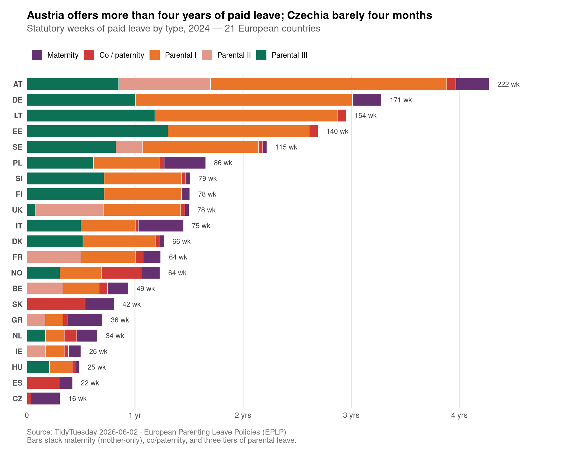

Reading the stacks

The same total bar length can come from very different policy mixes. Compare Poland (a thick maternity block, almost no parental tiers) with Estonia (essentially zero maternity, but two long parental tiers either parent can take). Two countries, similar total weeks, opposite philosophies of who the leave is for.

How did we get here?

The 2024 cross-section is a snapshot. The panel structure also lets us watch the policy mix evolve. Across the panel, the share of total leave that comes from parental tiers (rather than mother-only maternity) has risen steadily since the early 1990s — that is the structural story of European leave policy over the last three decades.

share_over_time <- eplp %>%
  transmute(
    country, year,
    maternity = mat_m_ld_bb + mat_m_ld_ab,
    parental  = par1_ld + par2_ld + par3_ld,
    copat     = co_ld
  ) %>%
  group_by(year) %>%
  summarise(
    maternity = mean(maternity),
    parental  = mean(parental),
    copat     = mean(copat),
    .groups = "drop"
  ) %>%
  pivot_longer(-year, names_to = "leave_type", values_to = "weeks") %>%
  mutate(
    leave_type = recode(
      leave_type,
      maternity = "Maternity",
      copat     = "Co / paternity",
      parental  = "Parental (all tiers)"
    ),
    leave_type = factor(
      leave_type,
      levels = c("Parental (all tiers)", "Maternity", "Co / paternity")
    )
  )

trend_cols <- palette_cols[c(3, 1, 2)]

p2 <- share_over_time %>%
  ggplot(aes(x = year, y = weeks, fill = leave_type)) +
  geom_area(alpha = 0.92, color = "white", linewidth = 0.25) +
  scale_fill_manual(values = trend_cols, name = NULL) +
  scale_x_continuous(breaks = seq(1970, 2024, 10),
                     expand = expansion(mult = c(0, 0))) +
  scale_y_continuous(expand = expansion(mult = c(0, 0.05))) +
  labs(
    title = "Parental leave overtook maternity leave as Europe's main entitlement",
    subtitle = "Average weeks of statutory paid leave across 21 European countries, 1970–2024",
    x = NULL,
    y = "Average weeks (panel mean)",
    caption = "Source: TidyTuesday 2026-06-02 · European Parenting Leave Policies (EPLP)"
  ) +
  theme_minimal(base_size = 12) +
  theme(
    plot.title = element_text(face = "bold", size = 13),
    plot.subtitle = element_text(color = "grey35",
                                 margin = margin(b = 12)),
    plot.caption = element_text(color = "grey45", hjust = 0,
                                margin = margin(t = 10)),
    panel.grid.minor = element_blank(),
    legend.position = "top",
    legend.justification = "left"
  )

p2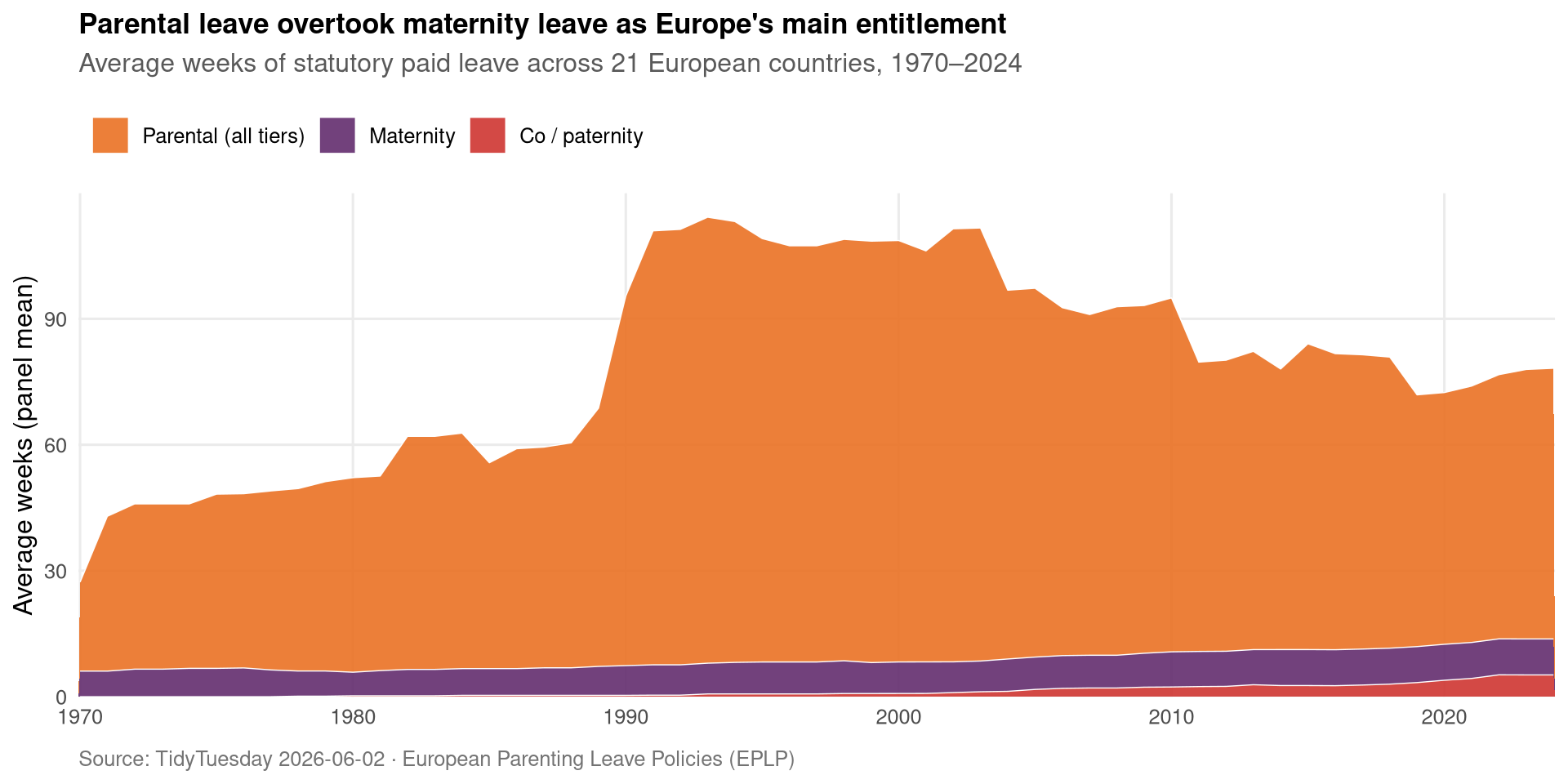

In 1970 the average European country in this panel offered roughly 12 weeks of paid leave, almost all of it medical maternity leave reserved for mothers. By 2024 the average has grown past 70 weeks, and the bulk of that growth is parental leave — entitlements that are increasingly designed to be transferable, shareable, or earmarked for the second parent. Co-leave (the small sliver at the top of each year) is a more recent invention, barely visible before the 2000s.

Final thoughts and takeaways

A few things stand out once the leave duration is decomposed rather than reported as a single “weeks of leave” headline:

Long totals are mostly parental, not maternity. The countries at the top of the 2024 ranking — Austria, Germany, Lithuania, Estonia — got there by stacking long parental-leave tiers, not by extending maternity leave. Maternity (mother-only, medical) has stayed in the 12–20 week range almost everywhere for thirty years.
The “second parent” is finally in the policy text. Co-leave/paternity was a rounding error in 1990 and is a small but persistent component by 2024. The shift toward leave that either parent can claim is even larger than the appearance of dedicated paternity weeks.
Policy on the books ≠ policy on the ground. This dataset is statutory entitlement, not take-up. A country that legislates 100 weeks of parental leave at a low replacement rate may see very different real behavior than one that offers 40 weeks at full pay. The *_rr (replacement rate) and *_cap fields in this panel are the natural next stop for anyone wanting to weight the durations by how usable the leave actually is.
The convergence is partial. Despite three decades of EU-level coordination, the spread between the most and least generous countries in 2024 is still enormous — Austria offers more than thirteen times the paid weeks Czechia does. Whatever harmonization pressure exists, it has not flattened the distribution.

For a household weighing where in Europe to start a family, the headline “weeks of leave” is the wrong number to compare. The right comparison is the mix: how much is reserved for the birthing parent, how much can be shared, how much is paid at what rate, and how much of it is realistically taken. This dataset is a clean foundation for that more careful comparison.