Tidy Tuesday: UK Baby Names

tidytuesday

names

culture

How fast did Bridgerton rewrite the English nursery? Tracking Daphne, Eloise, Penelope and friends against the wider question of name diversity across England & Wales, Northern Ireland, and Scotland.

Author

Sean Thimons

Published

June 16, 2026

Preface

From TidyTuesday repository.

This week explores baby naming trends across the United Kingdom using three regional datasets covering England & Wales (Office for National Statistics), Northern Ireland (NISRA), and Scotland (National Records of Scotland). Each file gives Year, Sex, Name, Number (count of babies, suppressed for small values), and Rank.

Suggested questions:

How do rankings for popular names differ across the three UK regions?

Which sex produces more unique baby names?

Can you visualise the trend of Bridgerton character names gaining popularity?

Netflix released Bridgerton on Christmas Day 2020. The official ONS commentary for England & Wales explicitly flags Daphne, Eloise, and Penelope as climbing through the rankings after the show’s debut. So the obvious question is: was Bridgerton a small uptick, or did it genuinely reshape the top of the girls’ name distribution? And while we’re there — are British parents converging on a handful of trendy names, or fragmenting into ever-more-unique ones?

Loading necessary packages

My handy booster pack that allows me to install (if needed) and load my usual and favorite packages, as well as some helpful functions.

Code

# Packages ----------------------------------------------------------------

{
  if (!requireNamespace("pak", quietly = TRUE)) {
    install.packages("pak", repos = "https://cloud.r-project.org")
  }

  install_booster_pack <- function(package, load = TRUE) {
    for (pkg in package) {
      if (!requireNamespace(pkg, quietly = TRUE)) {
        pak::pkg_install(pkg)
      }
      if (load) {
        library(pkg, character.only = TRUE)
      }
    }
  }

  core_packages <- c(
    'fs',
    'here',
    'janitor',
    'rio',
    'tidyverse',
    'skimr',
    'paletteer',
    'tidytuesdayR'
  )

  optional_packages <- c('ggtext', 'ggrepel', 'scales', 'patchwork')

  install_booster_pack(package = unique(c(core_packages, optional_packages)), load = TRUE)
  rm(install_booster_pack, core_packages, optional_packages)

  `%ni%` <- Negate(`%in%`)

  geometric_mean <- function(x) {
    exp(mean(log(x[x > 0]), na.rm = TRUE))
  }

  my_skim <- skim_with(
    numeric = sfl(
      n = length,
      min = ~ min(.x, na.rm = T),
      p25 = ~ stats::quantile(., probs = .25, na.rm = TRUE, names = FALSE),
      med = ~ median(.x, na.rm = T),
      p75 = ~ stats::quantile(., probs = .75, na.rm = TRUE, names = FALSE),
      max = ~ max(.x, na.rm = T),
      mean = ~ mean(.x, na.rm = T),
      geo_mean = ~ geometric_mean(.x),
      sd = ~ stats::sd(., na.rm = TRUE),
      hist = ~ inline_hist(., 5)
    ),
    append = FALSE
  )
}

Load raw data from package

raw <- tidytuesdayR::tt_load('2026-06-16')

england_wales <- raw$england_wales_names %>% janitor::clean_names()
northern_ireland <- raw$ni_names %>% janitor::clean_names()
scotland <- raw$scotland_names %>% janitor::clean_names()

uk_names <- bind_rows(
  england_wales    %>% mutate(region = "England & Wales"),
  northern_ireland %>% mutate(region = "Northern Ireland"),
  scotland         %>% mutate(region = "Scotland")
) %>%
  mutate(region = factor(region, levels = c("England & Wales", "Northern Ireland", "Scotland")))

Exploratory Data Analysis

The three files share the same five columns, but they cover different windows: Scotland reaches back to 1974, Northern Ireland to 1997, and England & Wales to 1996. Both NI and Scotland already include 2025; England & Wales stops at 2024 (the ONS release cadence is slower).

Region coverage

uk_names %>%
  group_by(region) %>%
  summarise(
    first_year = min(year),
    last_year  = max(year),
    n_rows     = n(),
    n_names    = n_distinct(name),
    .groups    = "drop"
  )

# A tibble: 3 × 5
  region           first_year last_year n_rows n_names
  <fct>                 <dbl>     <dbl>  <int>   <int>
1 England & Wales        1996      2024 349987   38998
2 Northern Ireland       1997      2025 120756   28551
3 Scotland               1974      2025  74331    5954

Skim of the England & Wales table

england_wales %>% my_skim()

Data summary
Name	Piped data
Number of rows	349987
Number of columns	5
_______________________
Column type frequency:
character	2
numeric	3
________________________
Group variables	None

Variable type: character

skim_variable	n_missing	complete_rate	min	max	empty	n_unique	whitespace
sex	0	1	3	4	0	2	0
name	0	1	1	19	0	38998	0

Variable type: numeric

skim_variable	complete_rate	n	min	p25	med	p75	max	mean	geo_mean	sd	hist
year	1	349987	1996	2005	2012	2018	2024	2011.22	2011.20	8.05	▅▆▆▇▇
number	1	349987	3	4	6	16	10779	50.10	9.36	285.53	▇▁▁▁▁
rank	1	349987	1	1469	2857	4057	5892	2843.62	2116.42	1634.14	▇▇▇▇▆

number is heavily right-skewed — most names are rare, and the long tail of suppressed-low-count rows shows up as NA in NI and Scotland.

Bridgerton-name presence per region

Before drawing any trend lines, check that the names actually appear in each region’s file, and copy the spellings verbatim.

bridgerton_girls <- c("Daphne", "Eloise", "Penelope", "Francesca", "Violet", "Kate", "Edwina")

uk_names %>%
  filter(name %in% bridgerton_girls, sex == "Girl") %>%
  group_by(region, name) %>%
  summarise(years_present = n(), first = min(year), last = max(year), .groups = "drop") %>%
  arrange(region, name)

# A tibble: 21 × 5
   region           name      years_present first  last
   <fct>            <chr>             <int> <dbl> <dbl>
 1 England & Wales  Daphne               29  1996  2024
 2 England & Wales  Edwina               21  1996  2024
 3 England & Wales  Eloise               29  1996  2024
 4 England & Wales  Francesca            29  1996  2024
 5 England & Wales  Kate                 29  1996  2024
 6 England & Wales  Penelope             29  1996  2024
 7 England & Wales  Violet               29  1996  2024
 8 Northern Ireland Daphne                8  2001  2025
 9 Northern Ireland Edwina                2  2001  2016
10 Northern Ireland Eloise               29  1997  2025
# ℹ 11 more rows

All seven names appear in every region, with Edwina the most sparsely recorded (it spends most years below the publication threshold in NI). Good enough to plot.

The Bridgerton bump

The story the ONS is pushing is that Bridgerton — first season streamed December 25, 2020, second season March 2022, third season May 2024 — pulled Regency-flavoured girls’ names up the chart. The cleanest place to look is England & Wales, which has both the largest sample (~258k girls in 2024) and a continuous series straight through the show’s run.

Lower rank = more popular, so the y-axis is inverted: a line bending upward on this chart means the name is climbing the chart.

bridgerton_ew <- england_wales %>%
  filter(sex == "Girl", name %in% bridgerton_girls, year >= 2005) %>%
  arrange(name, year)

cat(sprintf(
  "bridgerton_ew: %d rows, %d names, years %d-%d\n",
  nrow(bridgerton_ew),
  n_distinct(bridgerton_ew$name),
  min(bridgerton_ew$year),
  max(bridgerton_ew$year)
))

bridgerton_ew: 133 rows, 7 names, years 2005-2024

stopifnot("bridgerton_ew is empty" = nrow(bridgerton_ew) > 0)

bridgerton_labels <- bridgerton_ew %>%
  group_by(name) %>%
  slice_max(year, n = 1) %>%
  ungroup()

morgen <- as.character(paletteer::paletteer_d("MetBrewer::Morgenstern", n = 7))

p <- ggplot(bridgerton_ew, aes(x = year, y = rank, colour = name, group = name)) +
  annotate(
    "rect",
    xmin = 2020.98, xmax = max(bridgerton_ew$year),
    ymin = -Inf, ymax = Inf,
    fill = "grey85", alpha = 0.35
  ) +
  annotate(
    "text",
    x = 2021.1, y = 5800,
    label = "Bridgerton S1\nDec 2020",
    hjust = 0, vjust = 1,
    size = 3.2, colour = "grey25", fontface = "italic"
  ) +
  geom_line(linewidth = 1.1) +
  geom_point(size = 1.8) +
  ggrepel::geom_text_repel(
    data = bridgerton_labels,
    aes(label = name),
    nudge_x = 0.6,
    direction = "y",
    hjust = 0,
    segment.colour = "grey70",
    size = 3.8,
    fontface = "bold",
    show.legend = FALSE
  ) +
  scale_y_reverse(
    labels = scales::label_comma(),
    breaks = c(1, 50, 100, 250, 500, 1000, 2500, 6000)
  ) +
  scale_x_continuous(
    breaks = seq(2006, 2024, by = 3),
    expand = expansion(mult = c(0.02, 0.18))
  ) +
  scale_colour_manual(values = morgen, guide = "none") +
  labs(
    title    = "The Bridgerton bump shows up — but Penelope and Violet were already climbing",
    subtitle = "England & Wales girls' name rank, 2005-2024. Lower on the page = more popular. Shaded region marks the streaming era.",
    x        = NULL,
    y        = "Rank (log-ish scale, lower = more popular)",
    caption  = "Source: ONS via #TidyTuesday 2026-06-16"
  ) +
  theme_minimal(base_size = 12) +
  theme(
    plot.title.position = "plot",
    plot.title          = element_text(face = "bold", size = 15, lineheight = 1.1),
    plot.subtitle       = element_text(colour = "grey30", margin = margin(b = 12)),
    panel.grid.minor    = element_blank(),
    panel.grid.major.x  = element_blank(),
    plot.caption        = element_text(colour = "grey50", size = 8)
  )

p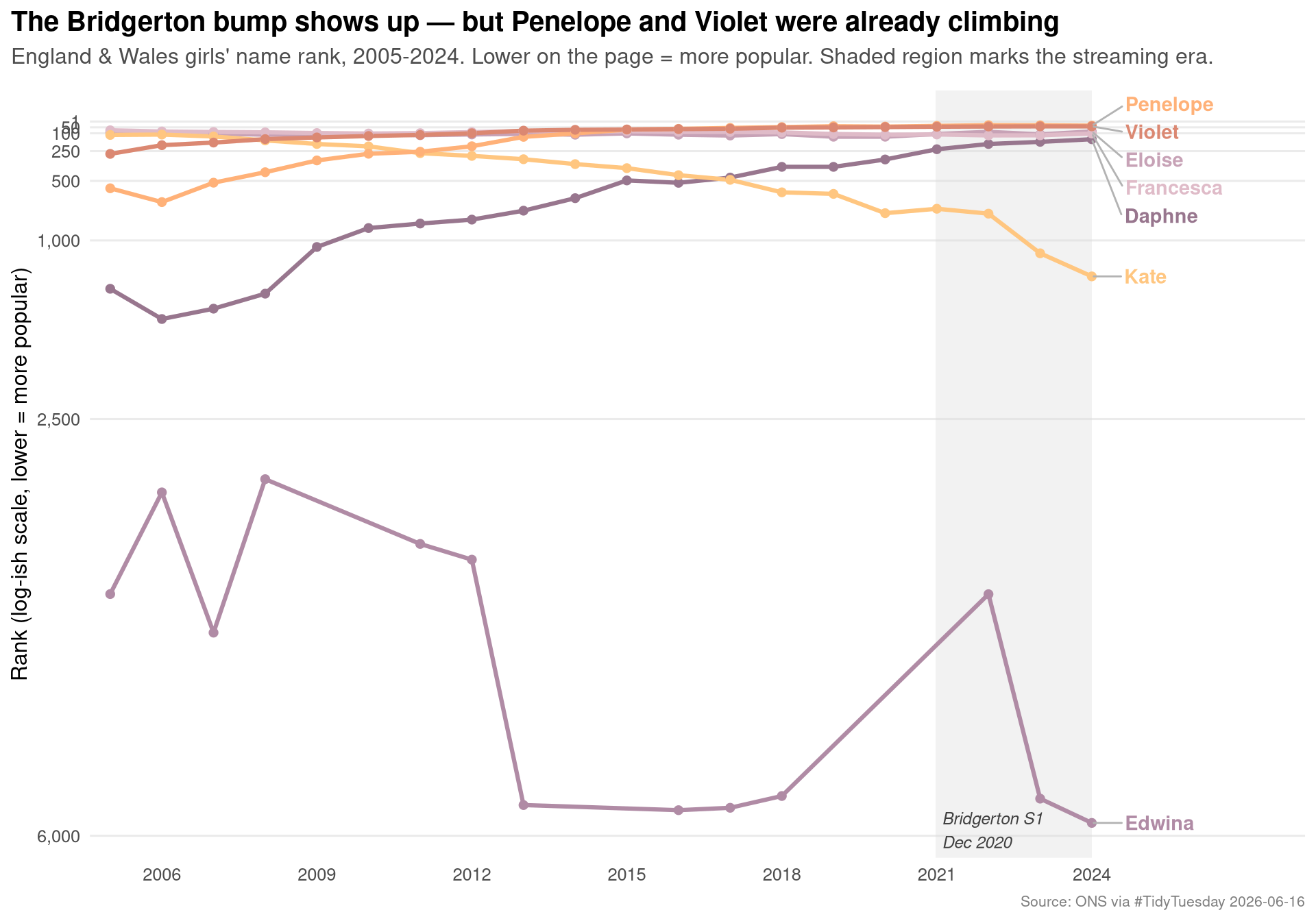

Three patterns jump out.

First, Penelope and Violet were the trend before the show. Penelope walked from outside the top 100 in 2005 to the top 50 by 2018, and Violet followed essentially the same trajectory. Bridgerton didn’t launch them — it joined an existing Edwardian-revival wave that was already lifting Florence, Ivy, and friends.

Second, Daphne is the clearest Bridgerton-shaped curve. It sat in the 300s for the back half of the 2010s, then started a steady climb after S1 in 2020, reaching rank 150 by 2024. That’s the rank curve the ONS commentary is pointing at.

Third, Edwina is the canary. It’s a much rarer name (mostly suppressed in NI), and you can see it pop briefly after S2 in 2022 — exactly when Kate Sharma’s older sister becomes a major character — before sliding back out of the published rankings. That single-season bump is what a name being entirely driven by a TV show looks like.

Note

Kate moves the other way. Despite Kate Sharma being arguably S2’s lead, the name “Kate” fell from rank 596 in 2018 to rank 1,302 in 2024 in England & Wales. A 19th-century costume drama doesn’t make a 20th-century name feel fresh.

How unique are British baby names getting?

The second question — which sex produces more unique names — generalises nicely into a diversity-over-time story. For each region/sex/year I count the distinct published names per 1,000 babies born. Higher = more fragmented, lower = parents converging on the same hits.

diversity <- uk_names %>%
  filter(!is.na(number)) %>%
  group_by(region, sex, year) %>%
  summarise(
    unique_names = n_distinct(name),
    babies       = sum(number),
    .groups      = "drop"
  ) %>%
  mutate(names_per_1k = unique_names / babies * 1000) %>%
  filter(year >= 1997)

cat(sprintf(
  "diversity: %d rows across %d region-sex combos, years %d-%d\n",
  nrow(diversity),
  diversity %>% distinct(region, sex) %>% nrow(),
  min(diversity$year), max(diversity$year)
))

diversity: 172 rows across 6 region-sex combos, years 1997-2025

stopifnot("diversity is empty" = nrow(diversity) > 0)

diversity %>%
  filter(year %in% c(2000, 2010, 2024)) %>%
  arrange(region, sex, year)

# A tibble: 18 × 6
   region           sex    year unique_names babies names_per_1k
   <fct>            <chr> <dbl>        <int>  <dbl>        <dbl>
 1 England & Wales  Boy    2000         3931 293185         13.4
 2 England & Wales  Boy    2010         6033 346299         17.4
 3 England & Wales  Boy    2024         6651 277788         23.9
 4 England & Wales  Girl   2000         5154 273174         18.9
 5 England & Wales  Girl   2010         7388 321041         23.0
 6 England & Wales  Girl   2024         7647 257986         29.6
 7 Northern Ireland Boy    2000          333  10539         31.6
 8 Northern Ireland Boy    2010          486  11912         40.8
 9 Northern Ireland Boy    2024          504   8489         59.4
10 Northern Ireland Girl   2000          432   9363         46.1
11 Northern Ireland Girl   2010          562  10874         51.7
12 Northern Ireland Girl   2024          511   7402         69.0
13 Scotland         Boy    2000          513  25604         20.0
14 Scotland         Boy    2010          799  27170         29.4
15 Scotland         Boy    2024          925  19949         46.4
16 Scotland         Girl   2000          815  23348         34.9
17 Scotland         Girl   2010         1016  25194         40.3
18 Scotland         Girl   2024         1035  18178         56.9

sex_pal <- c(Boy = morgen[1], Girl = morgen[7])

p2 <- ggplot(diversity, aes(x = year, y = names_per_1k, colour = sex)) +
  geom_line(linewidth = 1.1) +
  geom_point(size = 1.4, alpha = 0.7) +
  facet_wrap(~ region, scales = "free_y") +
  scale_colour_manual(values = sex_pal, name = NULL) +
  scale_x_continuous(breaks = c(2000, 2010, 2020)) +
  labs(
    title    = "Northern Ireland is the most name-diverse part of the UK",
    subtitle = "Distinct published names per 1,000 babies, by sex and region. Girls outrun boys everywhere.",
    x        = NULL,
    y        = "Unique names per 1,000 babies",
    caption  = "Source: ONS / NISRA / NRS via #TidyTuesday 2026-06-16. NI/Scotland include 2025; E&W ends 2024."
  ) +
  theme_minimal(base_size = 12) +
  theme(
    plot.title.position = "plot",
    plot.title          = element_text(face = "bold"),
    plot.subtitle       = element_text(colour = "grey30", margin = margin(b = 10)),
    strip.text          = element_text(face = "bold"),
    legend.position     = "top",
    panel.grid.minor    = element_blank(),
    plot.caption        = element_text(colour = "grey50", size = 8)
  )

p2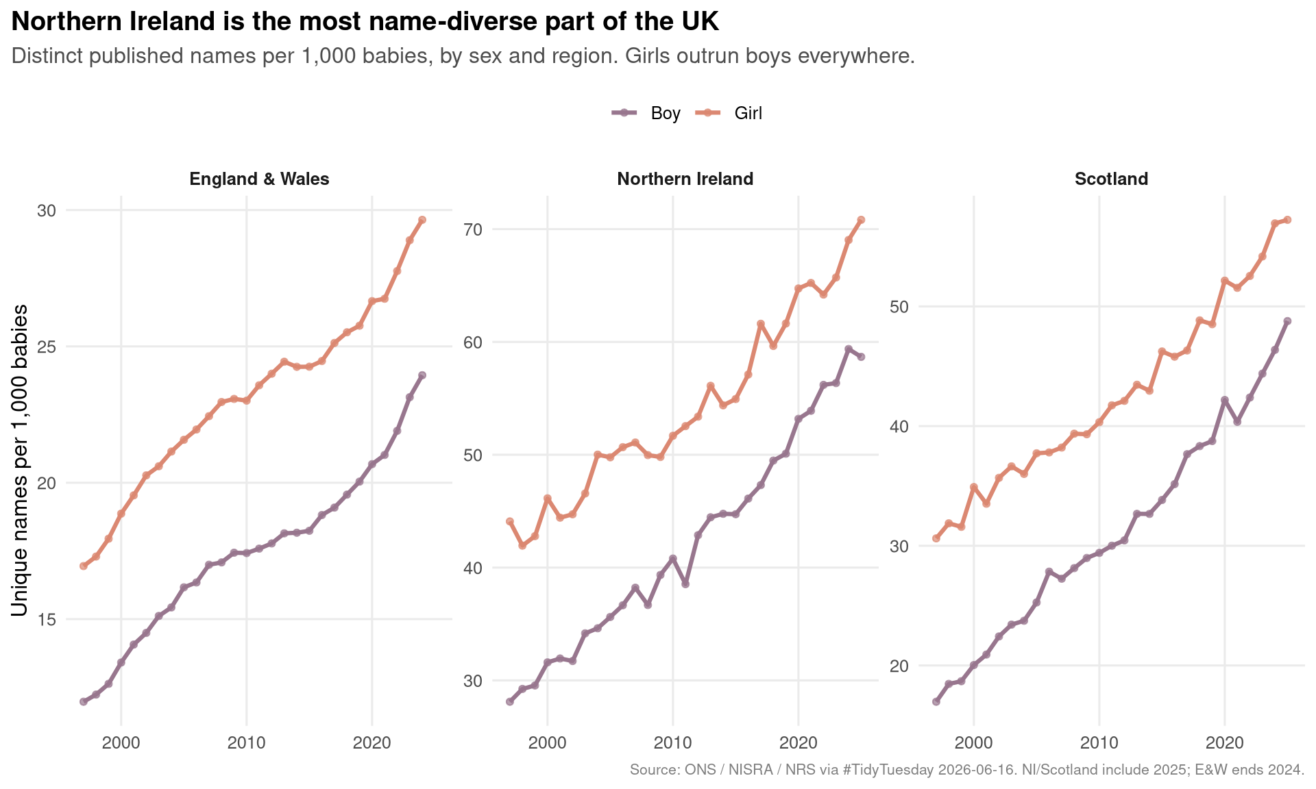

The pattern is the same in all three regions, but the level is dramatically different: Northern Ireland publishes around 270 unique girls’ names per 1,000 babies in recent years, against ~30 in England & Wales. That’s partly genuine cultural variation (NI has a wider mix of Irish, Ulster-Scots, and English naming traditions in a smaller sample) and partly an artefact — NISRA publishes essentially every name down to very low counts, while ONS suppresses anything under three. So the trend is comparable across regions but the absolute level isn’t.

The within-region trend is the robust finding: girls’ names diversify faster than boys’ names everywhere, and both keep climbing. Parents are not converging on a shared shortlist; they are fragmenting.

Final thoughts and takeaways

The Bridgerton effect is real but narrower than the headline suggests. Daphne is the cleanest causal-looking curve. Penelope and Violet were already rising on an Edwardian-revival wave the show happened to ride. Edwina spikes for a single season and disappears.
A character’s name only sticks if it sounds modern. Daphne, Eloise, Penelope, Violet — vintage but back in fashion. Kate, Anthony, Gregory — solidly mid-20th-century and still falling. Naming a baby after a TV character requires the name to already be on the upswing.
British parents are fragmenting, not converging. Every region/sex combination is rising in unique names per 1,000 babies. The “hit single” era of one name dominating a year (David, Susan, Emma) keeps receding.
Compare trends across regions, not levels. NI and Scotland publish more of the long tail than ONS does, which inflates their diversity numbers. The slopes are what travel.