Tidy Tuesday: UFC Athletes and Fight Data

UFC fight and athlete tables show a sport where the highlight reel is only one layer: modern records are roughly half decisions, half finishes, wrapped in profile labels that are more vocabulary than taxonomy.

Preface

From the TidyTuesday repository.

This week bundles several UFC tables from the fightr ecosystem: bout results, athlete profiles, ranking snapshots, betting-oriented features, and derived fight-level variables. I kept this pass descriptive. Combat-sports data are tempting prediction fuel, but the first question is simpler: what kind of sport is visible in the tables?

The answer is not quite the highlight reel. In these records, the UFC is a paired system: enough knockouts and submissions to keep the sport legible as danger, and enough decisions to remind us that the ordinary unit of analysis is often three or five rounds plus scorecards.

library(tidyverse)
library(tidytuesdayR)
library(scales)
library(patchwork)

raw <- tidytuesdayR::tt_load("2026-07-07")
ufc_fights <- raw$ufc_fights
ufc_athletes <- raw$ufc_athletes

fight_card <- list(
  paper = "#f8f3ea",
  ink = "#1d2329",
  muted = "#68717a",
  grid = "#d8c8ba",
  red = "#8f1d24",
  rust = "#bf5b35",
  amber = "#d99a3a",
  slate = "#34424f",
  cream = "#efe2cf"
)

theme_fight_card <- function(base_size = 12) {
  theme_minimal(base_size = base_size) +
    theme(
      plot.background = element_rect(fill = fight_card$paper, color = NA),
      panel.background = element_rect(fill = fight_card$paper, color = NA),
      panel.grid.major = element_line(color = fight_card$grid, linewidth = 0.25),
      panel.grid.minor = element_blank(),
      plot.title = element_text(face = "bold", color = fight_card$ink, margin = margin(b = 4)),
      plot.subtitle = element_text(color = fight_card$muted, margin = margin(b = 8)),
      plot.caption = element_text(color = fight_card$muted, hjust = 0, margin = margin(t = 8)),
      axis.title = element_text(color = fight_card$muted),
      axis.text = element_text(color = fight_card$ink),
      legend.position = "bottom",
      legend.title = element_text(color = fight_card$muted),
      legend.text = element_text(color = fight_card$ink),
      plot.margin = margin(8, 14, 8, 8)
    )
}

Coverage

Table	Rows
ufc_fights.csv	8,736
ufc_athletes.csv	3,145
Distinct outcome methods	10
Athletes with declared style labels	1,111

The promotion became a decision-and-finish machine

outcome_levels <- c("Decision", "KO/TKO", "Submission", "Administrative / other")

annual_outcomes <- ufc_fights %>%
  filter(!is.na(date), !is.na(method), method != "") %>%
  mutate(
    year = lubridate::year(date),
    outcome = case_when(
      str_detect(method, "Decision") ~ "Decision",
      method %in% c("KO/TKO", "TKO - Doctor's Stoppage") ~ "KO/TKO",
      method == "Submission" ~ "Submission",
      TRUE ~ "Administrative / other"
    )
  ) %>%
  count(year, outcome, name = "fights") %>%
  complete(
    year = full_seq(year, 1),
    outcome = outcome_levels,
    fill = list(fights = 0)
  ) %>%
  group_by(year) %>%
  mutate(
    year_total = sum(fights),
    share = if_else(year_total > 0, fights / year_total, NA_real_),
    outcome = factor(outcome, levels = rev(outcome_levels))
  ) %>%
  ungroup()

annual_totals <- annual_outcomes %>%
  distinct(year, year_total) %>%
  mutate(is_partial = year == max(year))

latest_full_year <- annual_totals %>%
  filter(year < max(year)) %>%
  filter(year == max(year)) %>%
  pull(year)

latest_labels <- annual_outcomes %>%
  filter(year == latest_full_year, outcome != "Administrative / other") %>%
  mutate(label = percent(share, accuracy = 1))

volume_plot <- ggplot(annual_totals, aes(year, year_total)) +
  annotate("rect", xmin = 1994, xmax = 2005.5, ymin = -Inf, ymax = Inf, fill = "#ffffff", alpha = 0.42) +
  annotate("rect", xmin = 2005.5, xmax = 2014.5, ymin = -Inf, ymax = Inf, fill = "#ead4c4", alpha = 0.38) +
  annotate("rect", xmin = 2014.5, xmax = Inf, ymin = -Inf, ymax = Inf, fill = "#d9e1df", alpha = 0.42) +
  geom_col(aes(fill = is_partial), width = 0.8, color = fight_card$paper, linewidth = 0.15) +
  scale_fill_manual(values = c(`FALSE` = fight_card$slate, `TRUE` = fight_card$amber), guide = "none") +
  scale_x_continuous(breaks = seq(1995, 2025, 5), expand = expansion(mult = c(0.01, 0.02))) +
  scale_y_continuous(labels = comma, expand = expansion(mult = c(0, 0.12))) +
  annotate("text", x = 1999.5, y = 585, label = "early archive\nsmall cards", color = fight_card$muted, size = 3.2, lineheight = 0.92) +
  annotate("text", x = 2010, y = 585, label = "expansion", color = fight_card$muted, size = 3.2) +
  annotate("text", x = 2020.5, y = 585, label = "modern volume", color = fight_card$muted, size = 3.2) +
  annotate("label", x = 2024.2, y = 315, label = "2026 is partial", label.size = 0, fill = "#fff6e5", color = fight_card$ink, size = 3.1) +
  labs(x = NULL, y = "Fights per year") +
  theme_fight_card(base_size = 11) +
  theme(
    axis.text.x = element_blank(),
    axis.title.y = element_text(margin = margin(r = 6)),
    panel.grid.major.x = element_blank(),
    plot.margin = margin(8, 22, 0, 8)
  )

heatmap_plot <- ggplot(annual_outcomes, aes(year, outcome, fill = share)) +
  annotate("rect", xmin = 1994, xmax = 2005.5, ymin = -Inf, ymax = Inf, fill = "#ffffff", alpha = 0.42) +
  annotate("rect", xmin = 2005.5, xmax = 2014.5, ymin = -Inf, ymax = Inf, fill = "#ead4c4", alpha = 0.38) +
  annotate("rect", xmin = 2014.5, xmax = Inf, ymin = -Inf, ymax = Inf, fill = "#d9e1df", alpha = 0.42) +
  geom_tile(color = fight_card$paper, linewidth = 0.35, width = 0.92, height = 0.82) +
  geom_text(
    data = latest_labels,
    aes(label = label),
    color = "white",
    fontface = "bold",
    size = 3.2
  ) +
  annotate(
    "label",
    x = 1997.4,
    y = 2.15,
    label = "The early table is\nmostly finishes",
    label.size = 0,
    fill = "#fff9f0",
    color = fight_card$ink,
    size = 3.2,
    lineheight = 0.92
  ) +
  annotate(
    "curve",
    x = 1998.7,
    xend = 1994.6,
    y = 2.45,
    yend = 2.95,
    curvature = 0.22,
    arrow = arrow(length = unit(0.10, "inches")),
    color = fight_card$red,
    linewidth = 0.45
  ) +
  annotate(
    "label",
    x = 2020.2,
    y = 4.35,
    label = "Recent full years sit\nnear a half-decision mix",
    label.size = 0,
    fill = "#fff9f0",
    color = fight_card$ink,
    size = 3.2,
    lineheight = 0.92
  ) +
  scale_fill_gradientn(
    colors = c("#f3e7d6", "#d99a3a", "#bf5b35", "#7f1d1d"),
    labels = percent,
    limits = c(0, 0.7),
    oob = squish,
    name = "Within-year share"
  ) +
  scale_x_continuous(breaks = seq(1995, 2025, 5), expand = expansion(mult = c(0.01, 0.02))) +
  labs(
    title = "The modern table is not finish-free. It is finish-and-decision balanced.",
    subtitle = "Outcome method by year, with fight volume above for sample-size context",
    x = NULL,
    y = NULL
  ) +
  coord_cartesian(clip = "off") +
  theme_fight_card(base_size = 12) +
  theme(
    panel.grid = element_blank(),
    axis.text.y = element_text(face = "bold"),
    legend.key.width = unit(1.25, "cm"),
    plot.margin = margin(0, 22, 8, 8)
  )

volume_plot / heatmap_plot + plot_layout(heights = c(0.55, 1.45))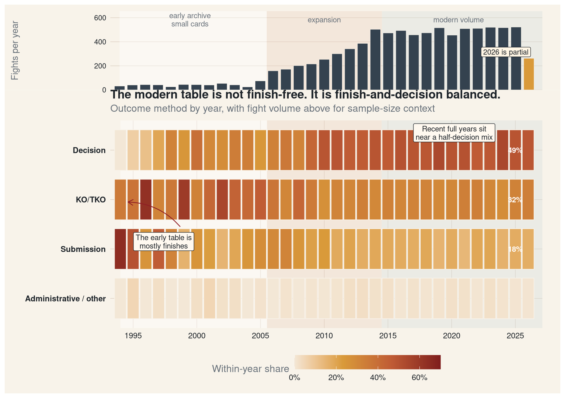

Figure 1: Annual fight volume and outcome share in the UFC bout table. The 2026 record is partial through late June; color shows within-year share, not an absolute count.

The simple method ranking was technically accurate, but it hid the key structure. Decisions are the largest single broad ending in the full fight table: 4,076 rows, or about 47% of fights. KO/TKO rows account for about 33%, and submissions about 19%. The useful claim is therefore not that finishes disappeared. They did not. The claim is that the mature table has settled into a roughly balanced braid of decisions and finishes.

That matters for analysis. A model trained on this table should not treat “finish” as the default shape of a fight. Nor should a story about UFC history pretend that every year is equally comparable: the early years are small, the middle years are a growth ramp, and 2026 is explicitly partial.

Style labels are profile vocabulary, not technical taxonomy

style_summary <- ufc_athletes %>%
  mutate(
    fighting_style = str_squish(fighting_style),
    fighting_style = na_if(fighting_style, ""),
    fighting_style = recode(fighting_style, `Kung-Fu` = "Kung Fu"),
    status = replace_na(status, "Unknown"),
    label_family = case_when(
      fighting_style %in% c("MMA", "Freestyle") ~ "umbrella label",
      fighting_style %in% c("Striker", "Grappler", "Brawler") ~ "role label",
      TRUE ~ "discipline label"
    )
  ) %>%
  filter(!is.na(fighting_style)) %>%
  group_by(fighting_style, label_family) %>%
  summarise(
    athletes = n(),
    active = sum(status == "Active"),
    active_share = active / athletes,
    .groups = "drop"
  ) %>%
  slice_max(athletes, n = 12) %>%
  arrange(athletes) %>%
  mutate(
    fighting_style = fct_inorder(fighting_style),
    active_label = str_glue("{comma(athletes)} total · {percent(active_share, accuracy = 1)} active")
  )

family_palette <- c(
  "umbrella label" = fight_card$red,
  "role label" = fight_card$rust,
  "discipline label" = fight_card$slate
)

ggplot(style_summary, aes(athletes, fighting_style)) +
  geom_rect(
    data = tibble(ymin = c(0.5, 2.5, 6.5), ymax = c(2.5, 6.5, 12.5)),
    aes(ymin = ymin, ymax = ymax),
    xmin = -Inf,
    xmax = Inf,
    inherit.aes = FALSE,
    fill = c("#ffffff", "#efe2cf", "#e4ece9"),
    alpha = 0.36
  ) +
  geom_col(aes(fill = label_family), width = 0.68, alpha = 0.92) +
  geom_segment(aes(x = active, xend = athletes, yend = fighting_style), color = "#fff1dc", linewidth = 0.9) +
  geom_point(aes(x = active), color = fight_card$ink, fill = fight_card$paper, shape = 21, size = 3.2, stroke = 0.9) +
  geom_text(aes(x = athletes + 15, label = active_label), hjust = 0, color = fight_card$muted, size = 3.1) +
  annotate(
    "label",
    x = 335,
    y = 8.8,
    label = "The largest labels are\numbrella descriptors,\nnot precise disciplines.",
    label.size = 0,
    fill = "#fff9f0",
    color = fight_card$ink,
    size = 3.25,
    lineheight = 0.94
  ) +
  scale_fill_manual(values = family_palette, name = NULL) +
  scale_x_continuous(labels = comma, expand = expansion(mult = c(0, 0.24))) +
  labs(
    title = "Profile styles read like scouting vocabulary",
    subtitle = "Total label counts with an active-roster marker",
    x = "Athletes with label",
    y = NULL
  ) +
  coord_cartesian(clip = "off") +
  theme_fight_card(base_size = 12) +
  theme(
    panel.grid.major.y = element_blank(),
    legend.position = "top",
    plot.margin = margin(8, 90, 8, 8)
  )

Figure 2: Top declared fighting-style labels in the UFC athlete profile table. The bar shows all athletes with that label; the dark marker shows currently active athletes.

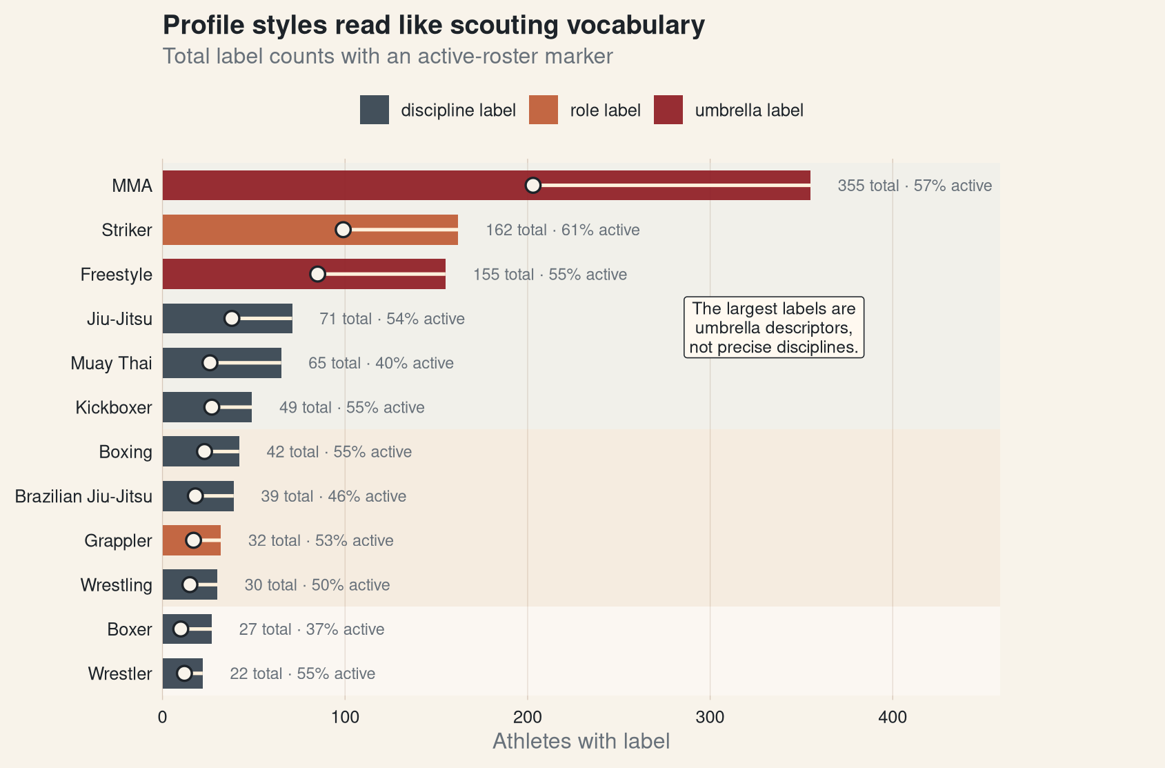
The style field is useful, but it is not a clean ontology. “MMA” and “Freestyle” are umbrella descriptors. “Striker” and “Grappler” are role labels. “Jiu-Jitsu,” “Muay Thai,” “Wrestling,” and “Judo” are closer to named disciplines, but the table mixes all of those vocabularies in one column.

That does not make the field useless. It means the field is better suited for exploratory grouping, quality checks, or reader-facing summaries than for hard technical inference. If I were modeling fight outcomes, I would keep profile style labels separate from measured fight actions, rankings, odds, and event history until the modeling question forced a join.

Takeaway

The useful story here is not “who will win.” It is that a modern fight dataset is a join of event history, athlete biographies, rankings, and market expectations. The outcome records say the sport is not reducible to highlights: decisions and finishes coexist at scale. The profile records say public labels are informative but messy.

That makes the dataset analytically rich, but easy to flatten incorrectly. Treat records, profiles, rankings, and odds as separate layers before collapsing them into one prediction table.