Tidy Tuesday: Many Penguins

A compact AVONET penguin trait table uses genus, sex labels, and morphology measurements to show how small biological datasets still carry structure.

Preface

From the TidyTuesday repository.

The many_penguins file is a small morphology slice from AVONET. It is compact enough to understand by inspection, but it carries the classic biological-data warning: the tidy table is not a sampling design. Species, genus, and sex labels are measurements and metadata, not guarantees of balanced coverage.

library(tidyverse)
library(tidytuesdayR)

raw <- tidytuesdayR::tt_load("2026-07-14")
many_penguins <- raw$many_penguins

Coverage

Measure	Value
Rows	93
Species	18
Genera	6
Usable beak/wing pairs	79

Taxonomic shape

many_penguins %>%
  count(genus, sort = TRUE) %>%
  mutate(genus = fct_reorder(genus, n)) %>%
  ggplot(aes(n, genus)) +
  geom_col(fill = "#1f6f8b") +
  labs(x = "Records", y = NULL) +
  theme_minimal(base_size = 12)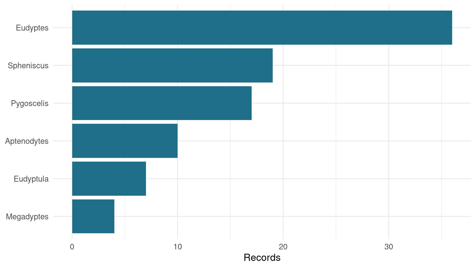

Figure 1: Penguin morphology records by genus.

The genus counts show the smallness of the file. This is not a citizen-science flood of repeated observations; it is a trait table. The unit of attention is the species/sex morphology record, so aggregation choices matter more than row count.

Sex labels

many_penguins %>%
  count(sex, sort = TRUE) %>%
  mutate(sex = fct_reorder(sex, n)) %>%
  ggplot(aes(n, sex, fill = sex)) +
  geom_col(width = 0.72, show.legend = FALSE) +
  geom_text(aes(label = n), hjust = -0.25, size = 4) +
  scale_fill_manual(values = c("F" = "#b56576", "M" = "#355070", "U" = "#6d597a")) +
  scale_x_continuous(expand = expansion(mult = c(0, 0.18))) +
  labs(x = "Records", y = NULL, title = "Unknown labels are visible evidence, not cleanup debris") +
  theme_minimal(base_size = 12) +
  theme(plot.title = element_text(face = "bold"))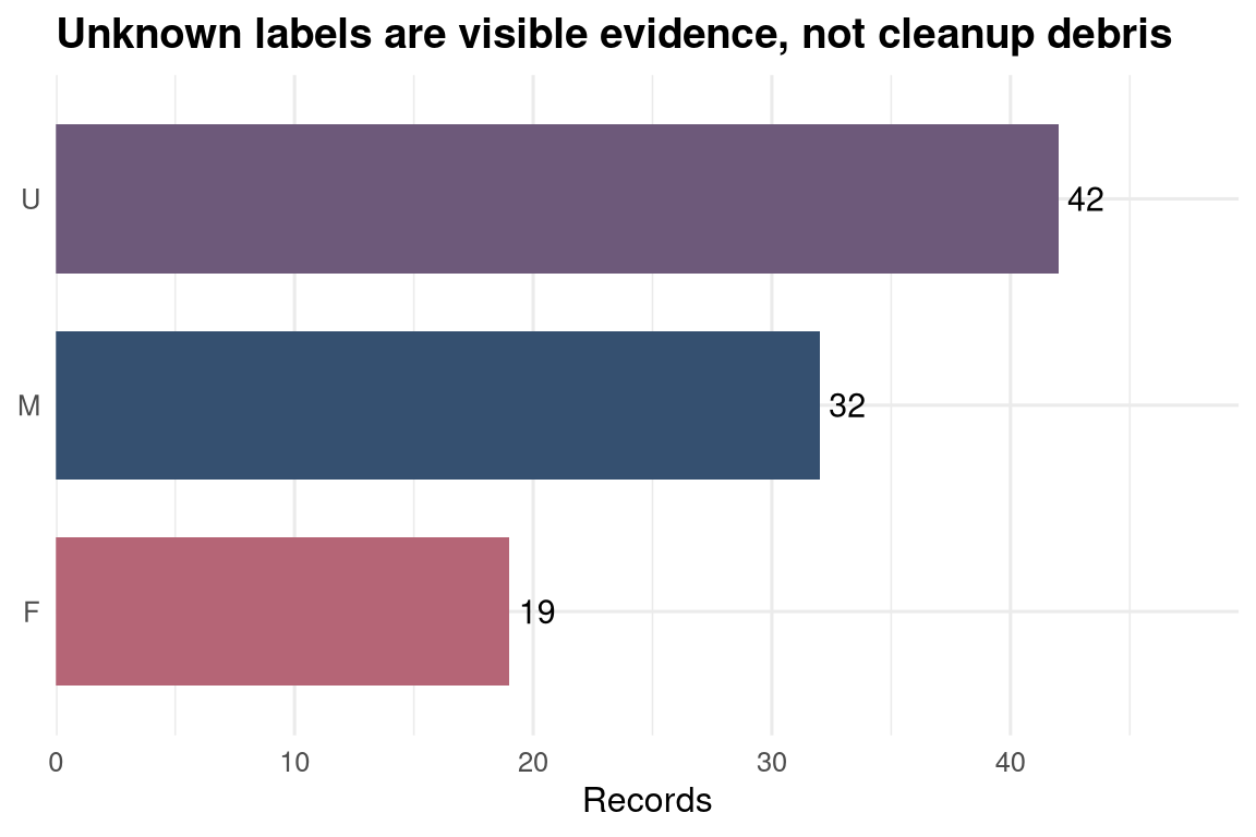

Figure 2: Sex labels preserve unknown or unsexed records rather than hiding them.

The U category is not a nuisance to delete. Unknown or unsexed records are part of the evidence trail. Dropping them would make the table look cleaner while silently changing the biological coverage.

Shape space

penguin_shape <- many_penguins %>%
  filter(!is.na(beak.length_culmen), !is.na(wing.length)) %>%
  select(genus, beak.length_culmen, wing.length)

stopifnot(nrow(penguin_shape) > 0)

# Fixed-scale small multiples expose within-genus spread without relying on color alone.
penguin_shape %>%
  ggplot(aes(beak.length_culmen, wing.length)) +
  geom_point(color = "#1f6f8b", size = 2.2, alpha = 0.8) +
  facet_wrap(vars(genus), ncol = 3) +
  labs(x = "Culmen length", y = "Wing length") +
  theme_minimal(base_size = 12)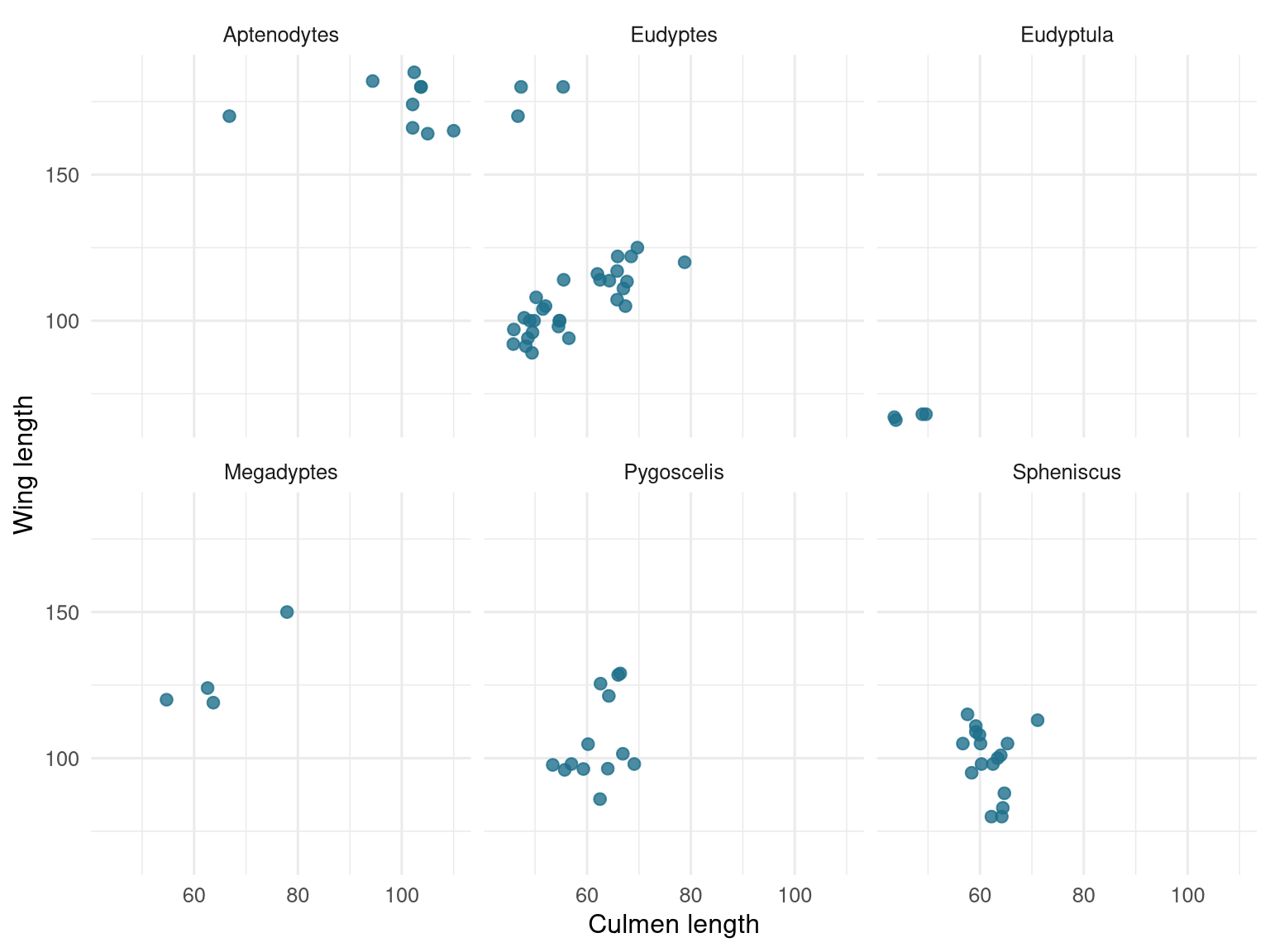

Figure 3: Culmen length and wing length sketch a quick morphology map.

The beak-wing small multiples are a quick morphology map. Keeping the same axes in every panel makes differences in body plan comparable, while separating genera reveals their internal spread without asking color alone to carry the grouping. Two measurements still do not summarize a bird, but they make the table’s structure legible.

Takeaway

This week is a good antidote to overbuilt dashboards. A few rows, clear trait columns, and a modest scatterplot are enough to ask better questions: Which genera are morphologically distinct? Which sex labels are comparable? Which measurements scale together, and which describe different ecological constraints?