Tidy Tuesday: Ecotourism

Gouldian finch records line up with a dry-season observation pattern, but the table records sightings, not bird abundance.

Preface

From the TidyTuesday repository.

This week’s files join ecological occurrences, Australian weather stations, and regional tourism estimates. I stayed with the Gouldian finch records because the date and nearest weather-station ID make a useful first question possible: what kind of weather sits behind the records that can be matched? The answer is mostly dry-season weather. It is not a claim about what finches prefer. A sighting is the result of a bird, a person or instrument, and a reporting system all meeting in one row.

Loading the data

if (!requireNamespace("pak", quietly = TRUE)) {
  install.packages("pak", repos = "https://cloud.r-project.org")
}

install_booster_pack <- function(package, load = TRUE) {
  for (pkg in package) {
    if (!requireNamespace(pkg, quietly = TRUE)) {
      pak::pkg_install(pkg)
    }
    if (load) {
      library(pkg, character.only = TRUE)
    }
  }
}

install_booster_pack(c("tidyverse", "tidytuesdayR", "paletteer", "scales"))
rm(install_booster_pack)

raw <- tidytuesdayR::tt_load("2026-07-28")
occurrences <- raw$occurrences
weather <- raw$weather

What is in the table

The occurrence file has 40,051 records. Orchids account for 35,052 of them, while the 3,922 Gouldian finch rows come from 57 nearest-station IDs. The weather file covers station days, not every observation. Joining by station and date leaves 2,117 finch records with usable temperature and rain fields.

Measure	Value
All occurrence records	40,051
Gouldian finch records	3,922
Finch records matched to usable daily weather	2,117
Distinct station-date pairs in the matched records	1,100

The dry-season observation pattern

month_order <- month.name

monthly_records <- finch_weather %>%
  mutate(
    month_name = factor(month.name[month], levels = month_order),
    weather = if_else(rainy == 1, "Rainy day", "Dry day")
  ) %>%
  count(month_name, weather) %>%
  complete(month_name, weather, fill = list(n = 0))

finch_weather %>%
  summarise(
    matched_records = n(),
    dry_records = sum(rainy == 0),
    dry_share = mean(rainy == 0),
    median_temperature = median(temp)
  )

# A tibble: 1 × 4
  matched_records dry_records dry_share median_temperature
            <int>       <int>     <dbl>              <dbl>
1            2117        1997     0.943               27.2

monthly_records %>%
  ggplot(aes(month_name, n, fill = weather)) +
  geom_col(width = 0.76) +
  scale_fill_manual(values = c("Dry day" = "#80521C", "Rainy day" = "#EBC174")) +
  scale_y_continuous(labels = comma, expand = expansion(mult = c(0, 0.08))) +
  labs(x = NULL, y = "Occurrence records", fill = NULL) +
  theme_minimal(base_size = 12) +
  theme(
    panel.grid.major.x = element_blank(),
    panel.grid.minor = element_blank(),
    axis.text.x = element_text(angle = 40, hjust = 1),
    legend.position = "top"
  )

Figure 1: Gouldian finch occurrence records with a matching weather row, by month and whether the nearest station recorded more than 5 mm of rain. These are record counts, not an estimate of finch abundance or a weather preference.

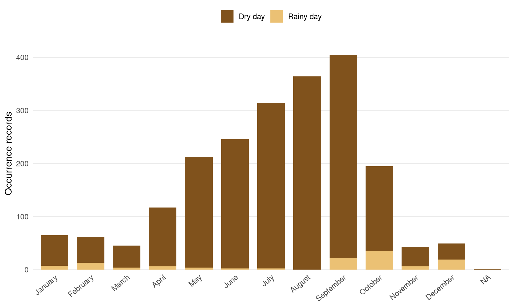
September has the largest count in the matched subset, with 405 records. July and August follow with 315 and 364. Across the full matched set, 94.3% of records fall on days the nearest station marks dry, and the median temperature is 27.2 C. That sounds tidy until you compare it with the raw calendar: the records also cluster around a handful of stations and years, especially 2022. Reporting effort has fingerprints.

A comparison that keeps the denominator visible

finch_station_days <- weather %>%
  filter(
    ws_id %in% unique(occurrences$ws_id[occurrences$organism_name == "Gouldian finch"]),
    !is.na(temp),
    !is.na(rainy)
  ) %>%
  transmute(temp, source = "All usable station days")

record_days <- finch_weather %>%
  transmute(temp, source = "Matched finch records")

bind_rows(finch_station_days, record_days) %>%
  ggplot(aes(temp, after_stat(density), fill = source, color = source)) +
  geom_density(alpha = 0.26, linewidth = 0.9) +
  geom_vline(xintercept = median(finch_weather$temp), color = "#3B2319", linewidth = 0.55, linetype = "22") +
  annotate(
    "text",
    x = median(finch_weather$temp) + 0.35,
    y = 0.072,
    label = paste0("record median: ", round(median(finch_weather$temp), 1), " C"),
    hjust = 0,
    color = "#3B2319",
    size = 3.4
  ) +
  scale_fill_manual(values = c("All usable station days" = "#D29C44", "Matched finch records" = "#80521C")) +
  scale_color_manual(values = c("All usable station days" = "#D29C44", "Matched finch records" = "#80521C")) +
  labs(x = "Daily average temperature (C)", y = "Density", fill = NULL, color = NULL) +
  theme_minimal(base_size = 12) +
  theme(
    panel.grid.minor = element_blank(),
    legend.position = "top"
  )

Figure 2: Temperature distribution for matched Gouldian finch records compared with all usable weather days at the 57 nearest stations represented in the finch file. The contrast gives context for the records, but it still cannot separate weather from observer effort, location, or season.

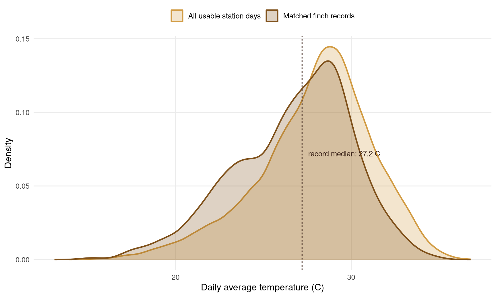
The weather-station comparison is useful because it prevents a familiar mistake: treating the records alone as the available conditions. Matched records have a mean temperature of 26.7 C, below the 27.9 C mean across usable days at those stations. Their rainy-day share is 5.7%, compared with 12.9% for the station-day file. Those differences describe the records in this dataset. They do not show that rain suppresses finch activity, or that 26.7 C is a biological optimum.

Takeaway

The ecotourism package makes a tempting promise: line up sightings, weather, and visitors, then tell a clean story about nature and travel. The joins are real, but the denominators are thin. This first pass finds a dry-season pattern among matched Gouldian finch records and shows why that pattern needs restraint. The next credible step would add observation effort or a survey design, then ask whether the same pattern survives.