
Tidy Tuesday: Basotho wool trade
tidytuesday
R
trade
lesotho
Monthly UN Comtrade records show a trade concentrated in South Africa and China, with a persistent dip during Lesotho’s winter months.
Preface
From the TidyTuesday repository.
This week’s file contains monthly mirror-import records for Lesotho’s raw wool and wool waste. The importing countries report the transactions, rather than Lesotho reporting its own exports. That distinction matters: this is a record of what partners entered into UN Comtrade, not a full production ledger or a direct measure of income reaching herders.
The file has 293 monthly records from 2010 through 2024. Four partners appear: South Africa, China, India, and Uruguay. The pattern is concentrated enough to make one question more interesting than the rest: when does the recorded trade happen, and who is doing the buying?
Loading necessary packages
Code
library(tidyverse)
library(janitor)
library(skimr)
library(tidytuesdayR)
library(paletteer)
library(scales)

`%ni%` <- Negate(`%in%`)

geometric_mean <- function(x) {
  exp(mean(log(x[x > 0]), na.rm = TRUE))
}

my_skim <- skim_with(
  numeric = sfl(
    n = length,
    min = ~ min(.x, na.rm = TRUE),
    p25 = ~ stats::quantile(.x, probs = .25, na.rm = TRUE, names = FALSE),
    med = ~ median(.x, na.rm = TRUE),
    p75 = ~ stats::quantile(.x, probs = .75, na.rm = TRUE, names = FALSE),
    max = ~ max(.x, na.rm = TRUE),
    mean = ~ mean(.x, na.rm = TRUE),
    geo_mean = ~ geometric_mean(.x),
    sd = ~ stats::sd(.x, na.rm = TRUE),
    hist = ~ inline_hist(.x, 5)
  ),
  append = FALSE
)
Load raw data from package
raw <- tidytuesdayR::tt_load("2026-08-04")
basotho_wool <- raw$basotho_wool
Exploratory data analysis
Basotho wool
basotho_wool %>%
  select(ref_year, ref_month, reporter_desc, qty, net_wgt, primary_value) %>%
my_skim()| Name | Piped data |
| Number of rows | 293 |
| Number of columns | 6 |
| _______________________ | |
| Column type frequency: | |
| character | 1 |
| numeric | 5 |
| ________________________ | |
| Group variables | None |
Variable type: character
| skim_variable | n_missing | complete_rate | min | max | empty | n_unique | whitespace |
|---|---|---|---|---|---|---|---|
| reporter_desc | 0 | 1 | 5 | 12 | 0 | 4 | 0 |
Variable type: numeric
| skim_variable | n_missing | complete_rate | n | min | p25 | med | p75 | max | mean | geo_mean | sd | hist |
|---|---|---|---|---|---|---|---|---|---|---|---|---|
| ref_year | 0 | 1 | 293 | 2010.00 | 2014.00 | 2018.0 | 2021 | 2024 | 2017.65 | 2017.64 | 4.27 | ▅▆▇▇▇ |
| ref_month | 0 | 1 | 293 | 1.00 | 3.00 | 6.0 | 9 | 12 | 6.13 | 4.95 | 3.41 | ▇▆▆▃▆ |
| qty | 1 | 1 | 293 | 0.00 | 34869.38 | 111754.5 | 445989 | 1719880 | 299283.28 | 111626.30 | 379348.01 | ▇▂▁▁▁ |
| net_wgt | 0 | 1 | 293 | 2.00 | 40132.29 | 114698.8 | 444958 | 1719880 | 302118.57 | 98914.10 | 376379.52 | ▇▂▁▁▁ |
| primary_value | 0 | 1 | 293 | 253.32 | 206087.01 | 662624.2 | 2129617 | 11107064 | 1595262.10 | 536540.22 | 2077526.37 | ▇▂▁▁▁ |
basotho_wool %>%
  summarise(
    records = n(),
    years = paste0(min(ref_year), "–", max(ref_year)),
    importing_partners = n_distinct(reporter_desc),
    quantity_estimates = sum(is_qty_estimated),
    weight_estimates = sum(is_net_wgt_estimated)
  )
# A tibble: 1 × 5
records years importing_partners quantity_estimates weight_estimates
<int> <chr> <int> <int> <int>
1 293 2010–2024 4 20 20Twenty records have estimated quantity and net weight fields, so I use primary_value for the main comparison. It is the UN Comtrade primary monetary value in US dollars and is present in every row. It should still be read as a transaction value, not a farm-gate price.
A small market with a strong calendar
month_labels <- month.abb

trade_by_month <- basotho_wool %>%
  group_by(ref_month) %>%
  summarise(
    value = sum(primary_value, na.rm = TRUE),
    observed_records = n(),
    .groups = "drop"
  ) %>%
  mutate(
    month = factor(month_labels[ref_month], levels = month_labels),
    season = if_else(ref_month %in% 6:8, "Southern winter", "Other months")
  )

trade_by_partner <- basotho_wool %>%
  group_by(reporter_desc) %>%
  summarise(
    value = sum(primary_value, na.rm = TRUE),
    kilograms = sum(net_wgt, na.rm = TRUE),
    .groups = "drop"
  ) %>%
  mutate(
    value_share = value / sum(value),
    reporter_desc = fct_reorder(reporter_desc, value)
  )

winter_totals <- trade_by_month %>%
  group_by(season) %>%
  summarise(value = sum(value), .groups = "drop")

winter_value <- winter_totals %>%
  filter(season == "Southern winter") %>%
  pull(value)

winter_share <- winter_value / sum(trade_by_month$value)

winter_fill <- "#74C8C3"
other_fill <- "#295384"
china_fill <- "#5A97C1"
south_africa_fill <- "#295384"
other_partner_fill <- "#95C36E"

monthly_plot <- ggplot(trade_by_month, aes(month, value, fill = season)) +
  geom_col(width = 0.78, color = "white", linewidth = 0.35) +
  geom_text(
    aes(label = comma(observed_records)),
    vjust = -0.35,
    size = 3.15,
    color = "grey35"
  ) +
  annotate(
    "rect", xmin = 5.5, xmax = 8.5, ymin = -Inf, ymax = Inf,
             fill = winter_fill, alpha = 0.12) +
  annotate(
    "text", x = 7, y = 7.1e7,
             label = paste0("Jun–Aug: ", dollar(winter_value, accuracy = 1e6),
                            " (", percent(winter_share, accuracy = 0.1), ")"),
             color = "#295384", fontface = "bold", size = 3.8) +
  scale_fill_manual(values = c("Other months" = other_fill, "Southern winter" = winter_fill)) +
  scale_y_continuous(labels = label_dollar(scale_cut = cut_short_scale()),
                     expand = expansion(mult = c(0, 0.14))) +
  labs(
    title = "Recorded wool trade thins out in Lesotho's winter",
    subtitle = "Total mirror-import value across 2010–2024; numbers above bars are observed partner-month records",
    x = NULL,
    y = "Reported primary value (USD)",
    fill = NULL
  ) +
  theme_minimal(base_size = 12) +
  theme(
    panel.grid.major.x = element_blank(),
    panel.grid.minor = element_blank(),
    plot.title = element_text(face = "bold", color = "#295384"),
    plot.subtitle = element_text(color = "grey35"),
    axis.text = element_text(color = "#295384"),
    axis.title = element_text(color = "#295384"),
    legend.position = "top"
  )

partner_plot <- ggplot(trade_by_partner, aes(value, reporter_desc, fill = reporter_desc)) +
  geom_col(width = 0.68, show.legend = FALSE) +
  geom_text(
    aes(label = percent(value_share, accuracy = 0.1)),
    hjust = -0.2,
    size = 3.8,
    color = "#295384",
    fontface = "bold"
  ) +
  scale_fill_manual(values = c(
    "South Africa" = south_africa_fill,
    "China" = china_fill,
    "India" = other_partner_fill,
    "Uruguay" = winter_fill
  )) +
  scale_x_continuous(labels = label_dollar(scale_cut = cut_short_scale()),
                     limits = c(0, 3.25e8), expand = expansion(mult = c(0, 0))) +
  labs(
    title = "Two buyers account for nearly all recorded value",
    subtitle = "Share of $467.4 million reported across the full file",
    x = "Reported primary value (USD)",
    y = NULL
  ) +
  theme_minimal(base_size = 12) +
  theme(
    panel.grid.major.y = element_blank(),
    panel.grid.minor = element_blank(),
    plot.title = element_text(face = "bold", color = "#295384"),
    plot.subtitle = element_text(color = "grey35"),
    axis.text = element_text(color = "#295384"),
    axis.title = element_text(color = "#295384")
  )

monthly_plot
partner_plot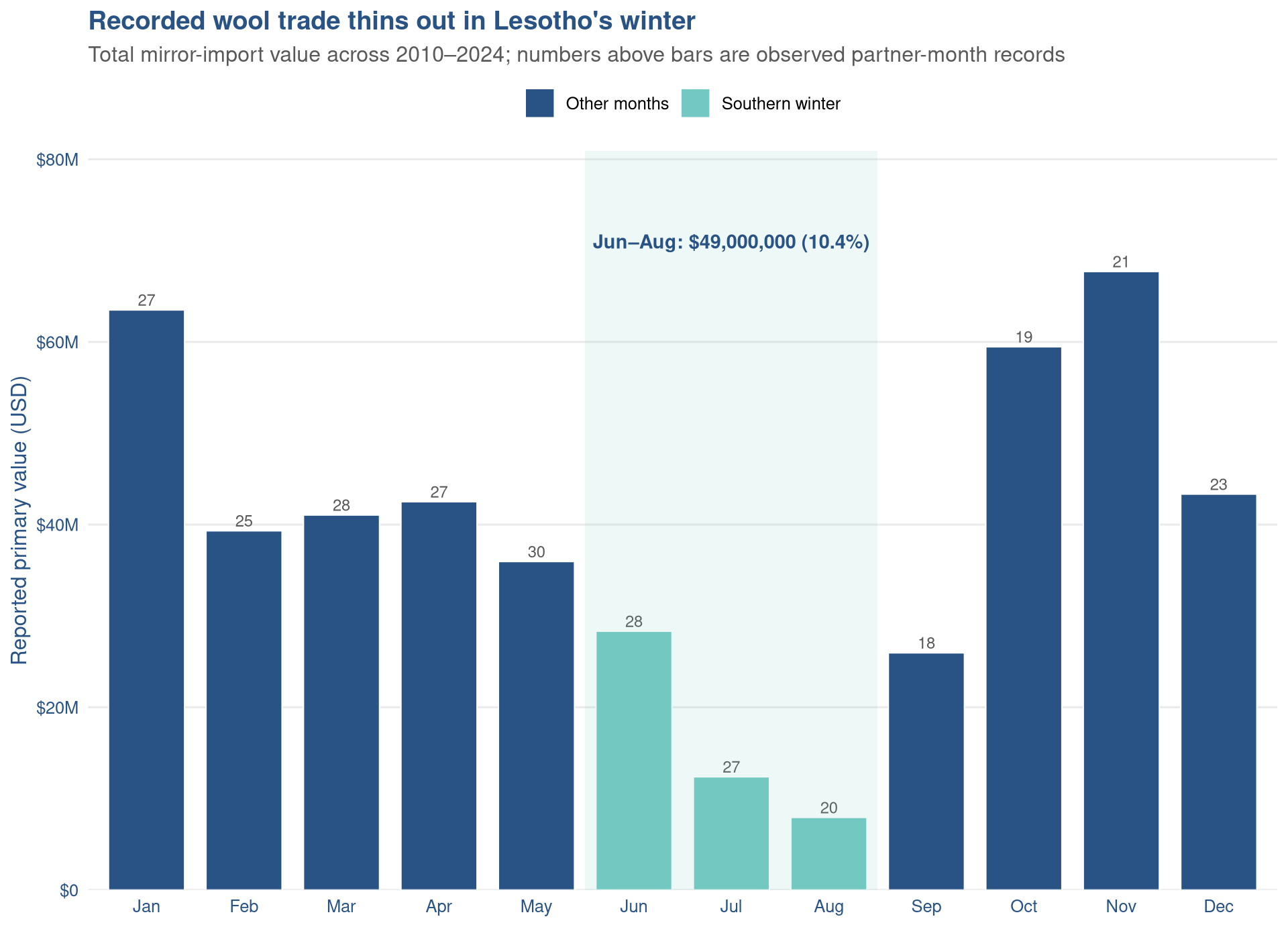
The winter signal is hard to miss. June through August make up $48.6 million, or 10.4% of the full-period value, even though those months supply 25.6% of the observed partner-month records. July and August are the two smallest months in the aggregate. This lines up with the seasonal question in the prompt, but it does not prove weather is the cause. Auction timing, transport, reporting practices, inventories, and the different dates at which buyers began reporting could all be part of the pattern.
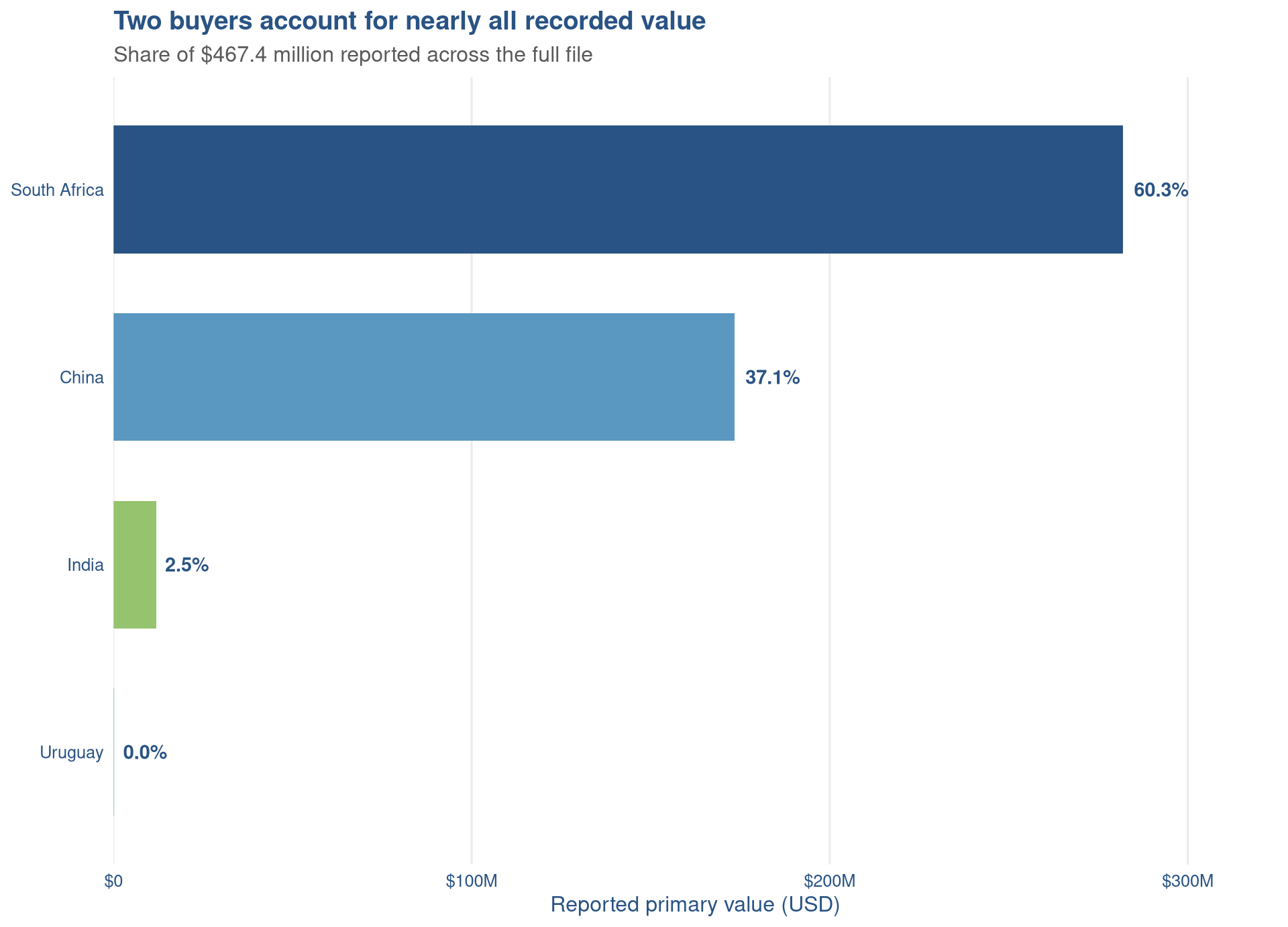
The market is also unusually concentrated. South Africa reported $281.9 million, or 60.3% of the file’s primary value, while China reported $173.4 million, or 37.1%. India and Uruguay together account for less than 3%. South Africa is the only partner present every year; China enters the file in 2016 and is already a large part of the 2024 total.
What the records can and cannot say
The dataset’s strength is its monthly detail. It shows that the trade calendar and the buyer list are both narrow enough to inspect directly. Its weak point is the denominator. There is no information here on total wool produced, stock held in Lesotho, shipment lead times, auction dates, or the value retained by producers.
That is why I would describe the chart as a reporting pattern, not a productivity story. The low winter total is a useful clue. It becomes an explanation only after it is matched with production, logistics, and auction data that are outside this file.
Final thoughts and takeaways
The Basotho wool records show a trade relationship built around two destinations and a clear seasonal lull. The most defensible result is modest: reported import value falls sharply in June through August, and South Africa plus China account for almost all value in the available records. The file points toward a question about the wool calendar; it does not settle why that calendar looks this way.