
Tidy Tuesday: Nearby galaxies do not hide the same kinds of nuclei
tidytuesday
R
astronomy
data-visualization
Palomar spectra show a sharp split between star-forming spiral nuclei and the LINER-heavy nuclei of early-type galaxies.
Preface
From the TidyTuesday repository.
The Palomar survey put a slit across the centers of 486 bright nearby galaxies and measured their optical spectra. A spectrum can tell a blunt but useful story about a galaxy’s nucleus. Young stars ionize gas one way. Accretion onto a black hole, shocks, and older stellar populations leave different ratios of oxygen, nitrogen, sulfur, and hydrogen lines.
The survey’s classification labels are already in the file, so this is not a new classifier. I wanted to see how much the mix of labels changes with the host galaxy’s visible morphology, then check that story against the classic BPT plane. The BPT diagram plots log([N II]/H-alpha) against log([O III]/H-beta). It is a diagnostic map, not a causal model.
Loading necessary packages
Code
library(tidyverse)
library(tidytuesdayR)
library(skimr)
library(scales)

`%ni%` <- Negate(`%in%`)
Load raw data from package
raw <- tidytuesdayR::tt_load("2026-08-11")
palomar_survey <- raw$palomar_survey
palomar_emission_lines <- raw$palomar_emission_lines
Exploratory data analysis
palomar_survey %>%
  select(activity_type, hubble_type, log_nii_ha, log_oiii_hb, velocity_dispersion_km_s) %>%
skim()| Name | Piped data |
| Number of rows | 486 |
| Number of columns | 5 |
| _______________________ | |
| Column type frequency: | |
| character | 2 |
| numeric | 3 |
| ________________________ | |
| Group variables | None |
Variable type: character
| skim_variable | n_missing | complete_rate | min | max | empty | n_unique | whitespace |
|---|---|---|---|---|---|---|---|
| activity_type | 71 | 0.85 | 4 | 10 | 0 | 5 | 0 |
| hubble_type | 0 | 1.00 | 1 | 16 | 0 | 304 | 0 |
Variable type: numeric
| skim_variable | n_missing | complete_rate | mean | sd | p0 | p25 | p50 | p75 | p100 | hist |
|---|---|---|---|---|---|---|---|---|---|---|
| log_nii_ha | 71 | 0.85 | 1.01 | 0.85 | 0.03 | 0.38 | 0.66 | 1.48 | 5.43 | ▇▃▁▁▁ |
| log_oiii_hb | 78 | 0.84 | 1.93 | 2.58 | 0.06 | 0.45 | 1.23 | 2.20 | 21.35 | ▇▁▁▁▁ |
| velocity_dispersion_km_s | 5 | 0.99 | 124.99 | 70.63 | 17.50 | 70.90 | 116.30 | 169.80 | 335.30 | ▇▇▅▂▁ |
palomar_survey %>%
  count(activity_type, sort = TRUE)
# A tibble: 6 × 2
activity_type n
<chr> <int>
1 H II 203
2 LINER 94
3 <NA> 71
4 Transition 65
5 Seyfert 52
6 Absorption 1There are 486 galaxies in the survey, but 71 have no activity label in this version of the data. Among the 415 labelled nuclei, H II regions make up 203 cases, LINERs 94, transitions 65, and Seyferts 52. The labels come with a warning label of their own: 84 classifications are uncertain or very uncertain. I keep them in the descriptive plots because they are part of the published catalogue, but I do not treat a hard boundary between colored points as a law of nature.
Morphology changes the mix
activity_levels <- c("H II", "Transition", "Seyfert", "LINER")
activity_colors <- c(
  "H II" = "#A65141",
  "Transition" = "#E7CDC2",
  "Seyfert" = "#80A0C7",
  "LINER" = "#394165"
)

morphology_mix <- palomar_survey %>%
  filter(activity_type %in% activity_levels) %>%
  mutate(
    morphology = case_when(
      str_detect(hubble_type, "^E") ~ "Elliptical",
      str_detect(hubble_type, "^S0") ~ "Lenticular",
      str_detect(hubble_type, "^S") ~ "Spiral",
      str_detect(hubble_type, "^I") ~ "Irregular",
      TRUE ~ "Other"
    )
  ) %>%
  count(morphology, activity_type) %>%
  group_by(morphology) %>%
  mutate(share = n / sum(n)) %>%
  ungroup() %>%
  mutate(
    morphology = factor(morphology, levels = c("Elliptical", "Lenticular", "Spiral", "Irregular", "Other")),
    activity_type = factor(activity_type, levels = activity_levels),
    label = if_else(share >= 0.10, percent(share, accuracy = 1), "")
  )

morphology_mix %>%
  ggplot(aes(morphology, share, fill = activity_type)) +
  geom_col(width = 0.72, color = "#FCF9F0", linewidth = 0.35) +
  geom_text(
    aes(label = label),
    position = position_stack(vjust = 0.5),
    color = "#17252f",
    fontface = "bold",
    size = 3.5
  ) +
  scale_fill_manual(values = activity_colors, name = "Nuclear label") +
  scale_y_continuous(labels = percent_format(), expand = expansion(mult = c(0, 0.03))) +
  labs(
    title = "Spiral nuclei are mostly H II, while LINER labels dominate early types",
    subtitle = "Shares within each broad morphology group; only labelled galaxies are included",
    x = NULL,
    y = "Share of labelled nuclei"
  ) +
  theme_minimal(base_size = 12) +
  theme(
    panel.grid.major.x = element_blank(),
    panel.grid.minor = element_blank(),
    plot.title = element_text(face = "bold"),
    legend.position = "top"
  )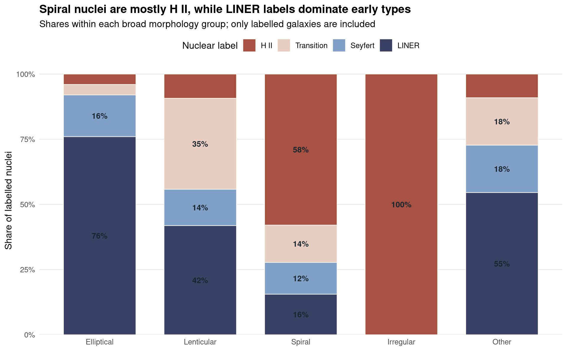
The contrast is large enough to see without statistical machinery. Of the 328 labelled spirals, 190 are H II nuclei, or 58%. The 25 labelled ellipticals point the other way: 19 are LINERs, or 76%. Lenticular galaxies sit between them, with LINER and transition labels together accounting for 77% of their labelled nuclei.
Those groups are uneven. Seven irregulars and 25 ellipticals are not much material for a general claim. The spiral result carries more weight because it has 328 labelled galaxies. It also has an obvious observational caution: a visual Hubble type is a broad description of the host, while a nuclear spectrum comes from a small central aperture.
The diagnostic map behind the labels
bpt_data <- palomar_survey %>%
  filter(
    activity_type %in% activity_levels,
    !is.na(log_nii_ha),
    !is.na(log_oiii_hb)
  ) %>%
  mutate(
    morphology = case_when(
      str_detect(hubble_type, "^E") ~ "Elliptical",
      str_detect(hubble_type, "^S0") ~ "Lenticular",
      str_detect(hubble_type, "^S") ~ "Spiral",
      str_detect(hubble_type, "^I") ~ "Irregular",
      TRUE ~ "Other"
    ),
    morphology = factor(morphology, levels = c("Elliptical", "Lenticular", "Spiral", "Irregular", "Other")),
    activity_type = factor(activity_type, levels = activity_levels)
  )

bpt_data %>%
  ggplot(aes(log_nii_ha, log_oiii_hb, color = activity_type)) +
  geom_vline(xintercept = -0.3, color = "grey70", linewidth = 0.35, linetype = "22") +
  geom_hline(yintercept = 0, color = "grey85", linewidth = 0.35) +
  geom_point(alpha = 0.72, size = 2.1) +
  facet_wrap(~ morphology, ncol = 3) +
  scale_color_manual(values = activity_colors, name = "Published label") +
  labs(
    title = "The morphology result survives a look at the line-ratio plane",
    subtitle = "Each point is a galaxy nucleus with both BPT coordinates",
    x = "log([N II] / H-alpha)",
    y = "log([O III] / H-beta)"
  ) +
  theme_minimal(base_size = 12) +
  theme(
    panel.grid.minor = element_blank(),
    plot.title = element_text(face = "bold"),
    legend.position = "top"
  )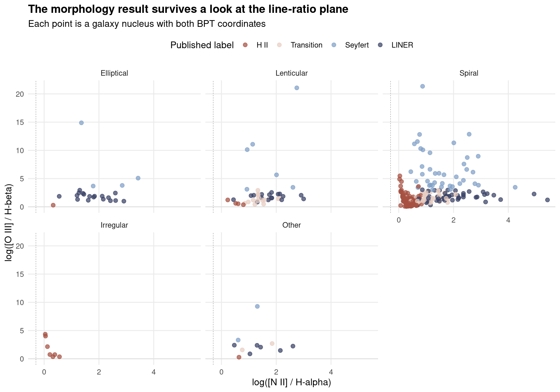
The BPT points do what the stacked bars suggested. H II nuclei in the spiral facet lean toward lower nitrogen-to-H-alpha ratios. LINER points occupy a different part of the plane and are common in the elliptical and lenticular facets. Seyferts overlap other labeled groups more than a simple two-cluster story would imply. That overlap is a useful reminder that the categories summarize line ratios and line profiles, not four sealed-off kinds of galaxies.
Final thoughts and takeaways
This small survey makes a strong descriptive point: nearby spiral galaxies and nearby early-type galaxies do not present the same menu of nuclear spectra. The clearest split is between H II labels in spirals and LINER labels in ellipticals and lenticulars. It does not tell us whether morphology caused that split, or whether every LINER line comes from the same physical process. The survey does give us a concrete place to start, with the raw line ratios still visible behind the catalog labels.