Getting started: a start-to-finish dose-response walkthrough

This vignette walks the Ward rotavirus human-challenge data from raw counts to a reported risk number, interpreting every output along the way. It answers two questions an end user actually has: what does my data need to look like going in, and what are the results saying coming out.

library(singlehit)

Load

The analysis needs three columns, one row per dose group: the administered dose, and the numbers of subjects who did (positive) and did not (negative) respond. The package ships this exact shape as ward_rotavirus:

data(ward_rotavirus)
ward_rotavirus
#> # A tibble: 8 × 3
#>        dose positive negative
#>       <dbl>    <dbl>    <dbl>
#> 1 90000            3        0
#> 2  9000            5        2
#> 3   900            7        1
#> 4    90            8        1
#> 5     9            8        3
#> 6     0.9          1        6
#> 7     0.09         0        7
#> 8     0.009        0        7

There are two ways in. The in-memory path standardizes a data frame you already have:

ward <- as_dose_response(ward_rotavirus)
ward
#> # A tibble: 8 × 5
#>        dose positive negative total response
#>       <dbl>    <dbl>    <dbl> <dbl>    <dbl>
#> 1     0.009        0        7     7    0    
#> 2     0.09         0        7     7    0    
#> 3     0.9          1        6     7    0.143
#> 4     9            8        3    11    0.727
#> 5    90            8        1     9    0.889
#> 6   900            7        1     8    0.875
#> 7  9000            5        2     7    0.714
#> 8 90000            3        0     3    1

The from-disk path reads the same data from the bundled text file — this is what you would use for your own delimited file:

ward_path <- system.file("extdata", "Ward_rotavirus.txt", package = "singlehit")
ward_from_file <- read_dose_response(ward_path)

identical(ward, ward_from_file)
#> [1] TRUE

Both routes produce the standardized dose · positive · negative · total · response tibble, where total = positive + negative and response = positive / total. The recognized aliases are dose, positive / pos / positive_response, and negative / neg / negative_response. Detection lowercases names and replaces punctuation with underscores, so Positive.Response is recognized. Rows sharing a dose are summed. Fitting requires at least 3 distinct doses and more than 1 total positive response — non-conforming data is rejected with an explanatory error.

Import a data frame or tribble

library(dplyr)
#> 
#> Attaching package: 'dplyr'
#> The following objects are masked from 'package:stats':
#> 
#>     filter, lag
#> The following objects are masked from 'package:base':
#> 
#>     intersect, setdiff, setequal, union

A data frame or a tibble from tibble::tribble() works the same way. Recognized aliases need no renaming:

counts <- data.frame(
  dose = c(1, 10, 100),
  pos = c(1, 5, 9),
  neg = c(9, 5, 1)
)
as_dose_response(counts)
#> # A tibble: 3 × 5
#>    dose positive negative total response
#>   <dbl>    <dbl>    <dbl> <dbl>    <dbl>
#> 1     1        1        9    10      0.1
#> 2    10        5        5    10      0.5
#> 3   100        9        1    10      0.9

Names such as dose_amount, infected, and uninfected are not recognized aliases. This table has valid values, but automatic column detection fails:

trial <- tibble::tribble(
  ~dose_amount, ~infected, ~uninfected,
             1,         1,           9,
            10,         5,           5,
           100,         9,           1
)
tryCatch(as_dose_response(trial), error = function(e) message(conditionMessage(e)))
#> Could not detect the dose column; supply its name explicitly.

Map the original names with quoted strings. This leaves trial unchanged and returns the standardized columns:

mapped <- as_dose_response(
  trial, dose = "dose_amount", positive = "infected", negative = "uninfected"
)
mapped
#> # A tibble: 3 × 5
#>    dose positive negative total response
#>   <dbl>    <dbl>    <dbl> <dbl>    <dbl>
#> 1     1        1        9    10      0.1
#> 2    10        5        5    10      0.5
#> 3   100        9        1    10      0.9

Or rename the columns before calling as_dose_response(). In dplyr::rename(), the new name goes on the left:

renamed <- trial %>%
  dplyr::rename(dose = dose_amount, positive = infected, negative = uninfected) %>%
  as_dose_response()
identical(mapped, renamed)
#> [1] TRUE

Mapping or renaming only fixes column detection. Doses must still be finite numeric values greater than zero, counts must be non-negative whole numbers, and every row must contain at least one subject. as_dose_response() also rejects fewer than three distinct doses or at most one positive response in total. A total column or a response proportion does not replace the required positive and negative counts.

Keep experiment details

A plain three-column data frame remains valid. You can also add study_id, host, dose_unit, and endpoint. Each supplied identity column must have one non-blank value across the table. study_id means an individual experiment; endpoint describes what was counted, while numeric response remains the observed proportion. Split experiments with different identities into separate tables before coercion.

example_path <- system.file("extdata", "dose-response-example.csv", package = "singlehit")
example_trial <- read_dose_response(example_path)
example_trial
#> # A tibble: 3 × 9
#>    dose positive negative total response study_id      host  dose_unit endpoint 
#>   <dbl>    <dbl>    <dbl> <dbl>    <dbl> <chr>         <chr> <chr>     <chr>    
#> 1     1        1        9    10      0.1 example_trial human FFU       infection
#> 2    10        5        5    10      0.5 example_trial human FFU       infection
#> 3   100        9        1    10      0.9 example_trial human FFU       infection

These example counts are illustrative. For your own experiment, find the blank CSV template with system.file("extdata", "dose-response-template.csv", package = "singlehit"), copy it into your working folder, and fill it in with a spreadsheet editor. Repeat experiment details on every row, enter counts and doses as numbers, and save as CSV. Read it with read_dose_response("my_trial.csv").

Additional metadata columns are preserved. Duplicate doses are combined only when their metadata agrees; conflicting values produce an error naming the column. total and response are recalculated from the counts.

Run

analyze_dose_response() does everything in one call: trend test, model fits, diagnostics, comparison, assessment, and bootstrap uncertainty. A fixed seed makes the bootstrap reproducible.

analysis <- analyze_dose_response(
  ward,
  bootstrap_times = 1000, # reduced for a fast vignette build; the default is 10000
  resample = "observed",
  seed = 2026
)

analysis
#> <qdr_analysis> microbial dose-response analysis
#> Trend: Z = 5.036, one-sided p = 2.38e-07
#> 
#> Model assessment:
#> # A tibble: 2 × 3
#>   model        recommendation  conclusion                                       
#>   <chr>        <chr>           <chr>                                            
#> 1 beta_poisson recommended     Beta-Poisson shows an adequate fit and is prefer…
#> 2 exponential  not_recommended Exponential does not show an adequate fit and is…
#> 
#> Model comparison:
#> # A tibble: 2 × 19
#>   model    parameters converged log_lik deviance   AIC   BIC delta_AIC delta_BIC
#>   <chr>         <int> <lgl>       <dbl>    <dbl> <dbl> <dbl>     <dbl>     <dbl>
#> 1 beta_po…          2 TRUE        -8.69     6.82  21.4  25.5        0         0 
#> 2 exponen…          1 TRUE       -72.6    135.   147.  149.       126.      124.
#> # ℹ 10 more variables: deviance_difference <dbl>, chi_square_df <int>,
#> #   chi_square_critical <dbl>, chi_square_p_value <dbl>,
#> #   significant_improvement <lgl>, preferred <lgl>, preferred_by_AIC <lgl>,
#> #   preferred_by_BIC <lgl>, selection <chr>, conclusion <chr>
#> 
#> Bootstrap replicates per model: 1000

The rest of this vignette unpacks each component of that qdr_analysis object.

Interpret each output

Trend — is there a dose-response signal at all?

analysis$trend
#> # A tibble: 1 × 5
#>   statistic     p_value alpha passes alternative
#>       <dbl>       <dbl> <dbl> <lgl>  <chr>      
#> 1      5.04 0.000000238  0.05 TRUE   increasing

dose_trend_test() runs a one-sided log-dose trend test. passes = TRUE means a monotonic increasing dose-response relationship was detected — response rises with dose.

What this is really saying: if passes were FALSE, there is no upward dose-response signal to model, and fitting mechanistic curves would not be warranted. Here it passes, so we proceed.

Goodness of fit — does each model fit the data at all?

analysis$goodness_of_fit
#> # A tibble: 2 × 8
#>   model    deviance    df critical_value  p_value good_fit assessment conclusion
#>   <chr>       <dbl> <int>          <dbl>    <dbl> <lgl>    <chr>      <chr>     
#> 1 exponen…   135.       7           14.1 6.92e-26 FALSE    inadequate Exponenti…
#> 2 beta_po…     6.82     6           12.6 3.38e- 1 TRUE     adequate   Beta-Pois…

This is the absolute check. Each model’s deviance is compared against a chi-squared critical_value; good_fit is TRUE when the deviance falls below it (equivalently, p_value > 0.05). assessment records adequate or inadequate.

What this is really saying: does this model describe the data acceptably on its own terms? A model can “win” a comparison and still fit badly — this is the gate that catches that.

Comparison — which model wins, and did the extra parameter earn its keep?

analysis$comparison
#> # A tibble: 2 × 19
#>   model    parameters converged log_lik deviance   AIC   BIC delta_AIC delta_BIC
#>   <chr>         <int> <lgl>       <dbl>    <dbl> <dbl> <dbl>     <dbl>     <dbl>
#> 1 beta_po…          2 TRUE        -8.69     6.82  21.4  25.5        0         0 
#> 2 exponen…          1 TRUE       -72.6    135.   147.  149.       126.      124.
#> # ℹ 10 more variables: deviance_difference <dbl>, chi_square_df <int>,
#> #   chi_square_critical <dbl>, chi_square_p_value <dbl>,
#> #   significant_improvement <lgl>, preferred <lgl>, preferred_by_AIC <lgl>,
#> #   preferred_by_BIC <lgl>, selection <chr>, conclusion <chr>

This is the relative check. The two-parameter Beta-Poisson is tested against the one-parameter Exponential (its nested limiting case) via the deviance_difference on the extra degree of freedom, alongside AIC/BIC and their deltas. significant_improvement and preferred flag the winner.

What this is really saying: the Beta-Poisson always fits at least as well because it has an extra parameter — significant_improvement asks whether that extra flexibility bought a statistically real improvement, or just curve-fit noise.

Assessment — the headline verdict

analysis$assessment[, c("model", "appropriate", "preferred", "recommendation", "conclusion")]
#> # A tibble: 2 × 5
#>   model        appropriate preferred recommendation  conclusion                 
#>   <chr>        <lgl>       <lgl>     <chr>           <chr>                      
#> 1 beta_poisson TRUE        TRUE      recommended     Beta-Poisson shows an adeq…
#> 2 exponential  FALSE       FALSE     not_recommended Exponential does not show …

build_model_assessment() fuses the absolute and relative checks into one recommendation label per model:

• recommended — fits adequately and is preferred.
• acceptable_alternative — fits adequately but is not preferred.
• preferred_but_inadequate — preferred but does not fit adequately (a red flag: the “best” model is still wrong).
• not_recommended — neither.

What this is really saying: this is the one row a risk assessor reads first. recommended means “use this model with confidence”; the conclusion column spells it out in plain language.

Consensus — an experimental cross-check

consensus_model_decision(analysis)
#> # A tibble: 2 × 13
#>   model     chi_squared_vote AIC_vote BIC_vote votes consensus_selected decision
#>   <chr>     <lgl>            <lgl>    <lgl>    <int> <lgl>              <chr>   
#> 1 beta_poi… TRUE             TRUE     TRUE         3 TRUE               selected
#> 2 exponent… FALSE            FALSE    FALSE        0 FALSE              not_sel…
#> # ℹ 6 more variables: agreement <chr>, criteria_available <int>,
#> #   chi_squared_choice <chr>, AIC_choice <chr>, BIC_choice <chr>,
#> #   conclusion <chr>

consensus_model_decision() treats the chi-squared, AIC, and BIC selections as three votes and reports the agreement level (unanimous, majority, or no_consensus).

What this is really saying: an experimental sanity check on the relative selection. It does not replace the absolute goodness-of-fit gate above — a unanimously-voted model can still fit inadequately.

Bootstrap intervals — the final risk numbers and their uncertainty

bootstrap_confint(analysis$bootstraps$beta_poisson, levels = c(0.95))
#> # A tibble: 4 × 5
#>   model        term  level  lower  upper
#>   <chr>        <chr> <dbl>  <dbl>  <dbl>
#> 1 beta_poisson alpha  0.95 0.161   0.707
#> 2 beta_poisson ed10   0.95 0.0766  0.790
#> 3 beta_poisson ed50   0.95 2.06   19.6  
#> 4 beta_poisson n50    0.95 2.06   19.6

The bootstrap refits the model to resampled data many times and reports percentile confidence intervals — not just for the parameters (alpha, n50) but for the effective doses ed10 and ed50: the doses producing a 10% and 50% response.

What this is really saying: these are the deliverable. ed50 is the median infectious dose; its interval is the honest uncertainty around it, driven by how much data you have and how noisy it is.

Plots

autoplot() on the analysis shows each fitted curve over the observed points:

ggplot2::autoplot(analysis)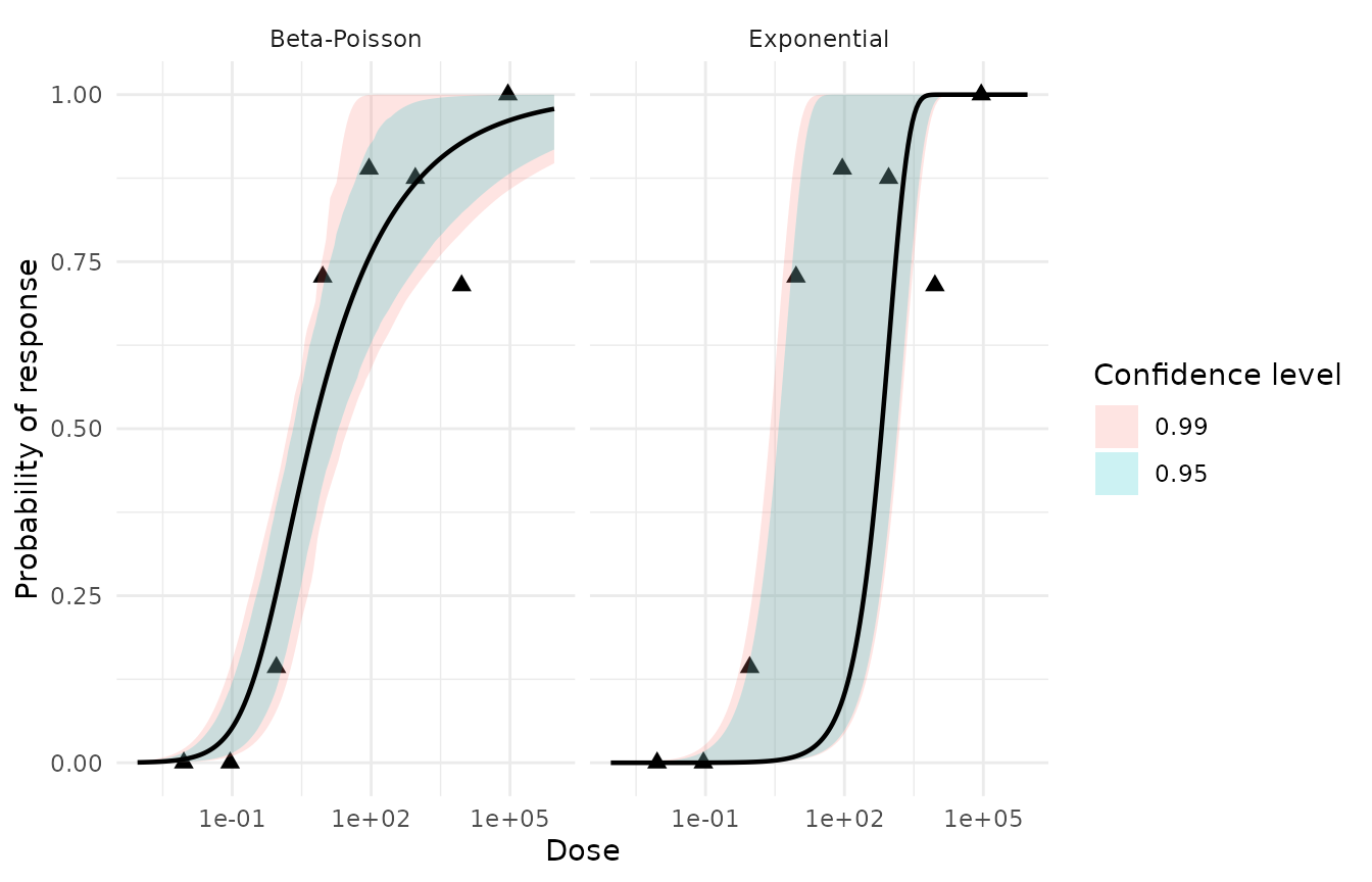

autoplot() on a bootstrap object shows the sampling distribution of the fitted parameters — the visual form of the intervals above:

ggplot2::autoplot(analysis$bootstraps$beta_poisson)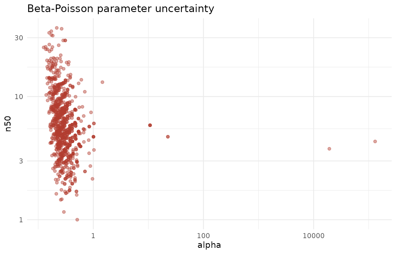

The final answer

Read the recommended model’s ed50 and its interval, and you have the number a risk assessor reports:

# Which model did the assessment recommend?
recommended <- analysis$assessment$model[analysis$assessment$recommendation == "recommended"][1]
recommended
#> [1] "beta_poisson"

# Its bootstrap intervals, then keep only the ed50 row.
ci <- bootstrap_confint(analysis$bootstraps[[recommended]], levels = c(0.95))
ci[ci$term == "ed50", ]
#> # A tibble: 1 × 5
#>   model        term  level lower upper
#>   <chr>        <chr> <dbl> <dbl> <dbl>
#> 1 beta_poisson ed50   0.95  2.06  19.6

That single row — the median infectious dose of the recommended model with its 95% percentile interval — is the deliverable: the dose at which half of exposed subjects are expected to be infected, with a defensible bound on how sure we are.

Which experiments can be pooled?

Use the bundled synthetic collection to try pooling before using your own studies. It contains three artificial experiments, A, B, and C, with the same host, dose unit, and infection endpoint. Each experiment has four doses and 100 subjects per dose. A and B have similar curves; C has a lower response. These are teaching data, not observations from a real pathogen.

Read and split the collection

pooling_path <- system.file("extdata", "pooling-example.csv", package = "singlehit")
raw_trials <- readr::read_csv(pooling_path, show_col_types = FALSE)
collection <- list(
  pathogen = "Synthetic example",
  datasets = split(raw_trials, raw_trials$study_id)
)
names(collection$datasets)
#> [1] "A" "B" "C"

The output names A, B, and C. Keep the pathogen name once on the collection. Split by study_id before coercion because it identifies an individual experiment. read_dose_response() handles one experiment at a time and rejects mixed identity values. Check that hosts, units, and endpoints match before pooling; the current pooling functions do not enforce that comparison.

Inspect every combination

report <- poolability_combinations(collection$datasets)
report[c("combination", "model", "p_value", "poolable", "converged")]
#> # A tibble: 8 × 5
#>   combination model         p_value poolable converged
#>   <chr>       <chr>           <dbl> <lgl>    <lgl>    
#> 1 A + B       exponential  9.40e- 1 TRUE     TRUE     
#> 2 A + B       beta_poisson 9.25e- 1 TRUE     TRUE     
#> 3 A + C       exponential  2.50e-66 FALSE    TRUE     
#> 4 A + C       beta_poisson 9.60e-62 FALSE    TRUE     
#> 5 B + C       exponential  4.06e-67 FALSE    TRUE     
#> 6 B + C       beta_poisson 4.31e-62 FALSE    TRUE     
#> 7 A + B + C   exponential  5.24e-87 FALSE    TRUE     
#> 8 A + B + C   beta_poisson 1.19e-79 FALSE    TRUE

Each row tests one combination under one model. At the default alpha = 0.05, A+B passes under both models, with p-values around 0.94 and 0.93. Every combination containing C fails. All fits converged, so this example has no optimizer failure flags.

poolable = TRUE means the test did not detect a significantly worse fit when sharing one parameter set. It does not prove equivalence or adequate absolute model fit. A passing pair can fail after another experiment is added, so read the row for the complete combination you plan to pool. These are exploratory p-values without multiple-testing adjustment.

Select non-overlapping groups

groups <- group_datasets(collection$datasets, method = "exhaustive")
groups
#> # A tibble: 6 × 3
#>   dataset model        group
#>   <chr>   <chr>        <int>
#> 1 A       exponential      1
#> 2 B       exponential      1
#> 3 C       exponential      2
#> 4 A       beta_poisson     1
#> 5 B       beta_poisson     1
#> 6 C       beta_poisson     2

A and B share group 1; C is in group 2 for both models. Group numbers are labels, not rankings. The exhaustive method considers all divisions into groups and returns one selected grouping per model. The default agglomerative method instead merges compatible groups greedily. Exhaustive grouping and combination reporting both default to a maximum of six experiments.

You can also inspect just the proposed A+B pool:

pair <- poolability_test(collection$datasets[c("A", "B")])
pair[c("model", "p_value", "poolable", "converged", "conclusion")]
#> # A tibble: 2 × 5
#>   model        p_value poolable converged conclusion                            
#>   <chr>          <dbl> <lgl>    <lgl>     <chr>                                 
#> 1 exponential    0.940 TRUE     TRUE      The datasets are poolable under the E…
#> 2 beta_poisson   0.925 TRUE     TRUE      The datasets are poolable under the B…

For this example, A and B are candidates for a shared fit; keep C separate. The report and grouping functions test poolability and return assignments. They do not create a pooled analysis or establish goodness of fit. A later pooled fit must preserve separate trial observations at repeated doses; simply coercing stacked trials would aggregate those observations or reject mixed identities.