Pooling experiments: tests, heatmaps, and forking paths
Source:vignettes/articles/pooling.Rmd
pooling.RmdWhen several challenge studies exist for one pathogen, it is tempting to combine them into one dose-response curve: more subjects, narrower intervals, one number to report. singlehit’s pooling functions test whether that is defensible. This article explains what the tests do, how to read their results, and how to avoid the main trap, which is letting the test results choose the groups.
The data
The bundled file holds six human Cryptosporidium challenge experiments compiled by the QMRA wiki. Every experiment used healthy adult volunteers, oral exposure, and doses counted in oocysts. Most differ in the parasite isolate, and one records a different outcome.
path <- system.file("extdata", "cryptosporidium-isolates.csv", package = "singlehit")
raw <- readr::read_csv(path, show_col_types = FALSE, col_types = readr::cols(study_id = "c"))
unique(raw[c("study_id", "isolate", "endpoint", "source")])
#> # A tibble: 6 × 4
#>   study_id isolate         endpoint  source
#>   <chr>    <chr>           <chr>     <chr>
#> 1 108      Iowa strain     infection DuPont et al. (1995)
#> 2 139      Iowa isolate    infection Messner et al. (2001)
#> 3 140      TAMU isolate    infection Messner et al. (2001)
#> 4 141      UCP isolate     infection Messner et al. (2001)
#> 5 181      TU502           diarrhea  Chappell et al. (2006)
#> 6 183      Moredun isolate infection Okhuysen et al. (2002)
trials <- split(raw, raw$study_id)
Each experiment has four to eight dose groups with a handful of volunteers in each. That small size matters for everything below.
What a poolability test asks
poolability_test() runs the likelihood-ratio test
described by Haas, Rose, and Gerba. For a set of experiments it:
- fits each experiment separately and adds up their deviances (the lack of fit);
- stacks every experiment’s dose groups and fits one shared curve;
- takes the difference in deviance as the test statistic. Sharing one curve can only fit as well or worse, so the statistic is never negative;
- compares it with a chi-squared distribution whose degrees of freedom are the parameters saved by sharing: one per extra experiment for the exponential model (k), two per extra experiment for beta-Poisson (alpha and N50).
The p-value answers one narrow question: if these experiments really shared one curve, how surprising would this much extra lack of fit be? A small p-value is evidence that they do not share a curve. A large one only means the data could not tell them apart.
Decide the groups first
The grouping should come from what the experiments are, decided before looking at any test: same pathogen and isolate, same outcome, same host and route, same dose unit. For these data the isolate is the obvious candidate, because isolates of Cryptosporidium are known to differ in infectivity.
singlehit enforces one of these conditions itself. Doses in different
units are not comparable, so datasets that record different
dose_unit values are refused:
relabelled <- trials[c("139", "140")]
relabelled[["140"]]$dose_unit <- "genome copies"
tryCatch(poolability_test(relabelled), error = conditionMessage)
#> [1] "Datasets record different dose units, so their doses are not comparable: '139' (oocysts), '140' (genome copies). Pool only datasets that share a unit."
Hosts, routes, isolates, and outcomes are not checked. Comparing them is your job.
A prespecified test
Messner and colleagues (2001) analysed three isolates challenged in the same programme: Iowa (139), TAMU (140), and UCP (141). A natural prespecified question is whether the three isolates share one curve.
isolates <- poolability_test(trials[c("139", "140", "141")])
isolates[c("model", "lrt_statistic", "df", "p_value", "converged")]
#> # A tibble: 2 × 5
#>   model        lrt_statistic    df  p_value converged
#>   <chr>                <dbl> <int>    <dbl> <lgl>
#> 1 exponential           79.2     2 6.18e-18 TRUE
#> 2 beta_poisson          10.3     4 3.57e- 2 TRUE
Pooling is rejected under both models (exponential p < 0.001, beta-Poisson p = 0.036). The separate fits show why: the isolates differ several-fold in median infectious dose.
n50 <- vapply(c("139", "140", "141"), function(id) {
  fit <- fit_dose_response(trials[[id]], "beta_poisson")
  generics::tidy(fit)$estimate[generics::tidy(fit)$term == "n50"]
}, numeric(1))
round(n50)
#> 139 140 141
#>  78   9 179
The defensible conclusion is to model the isolates separately, or to
model the variation between them explicitly (Messner and colleagues used
a hierarchical model for exactly this), rather than to report one pooled
curve. Had the test not rejected pooling,
fit_pooled_dose_response() would fit the shared curve to
the stacked dose groups.
Exploring every pair
Sometimes you want to see the structure first: which experiments look
alike? group_datasets() tests every pair and then proposes
a grouping. The pairwise p-values are attached to its result.
The two group_datasets() searches in this article take
about a minute together, so their results were computed ahead of time by
data-raw/pooling-article-results.R and are read from a
saved file; everything else runs as the article is built.
# Collect the convergence warnings rather than printing one per refit.
warnings <- character()
explore <- withCallingHandlers(
  group_datasets(trials, method = "agglomerative"),
  warning = function(w) {
    warnings <<- c(warnings, conditionMessage(w))
    invokeRestart("muffleWarning")
  }
)
unique(warnings)
pairwise <- attr(explore, "pairwise")
#> [1] "The Beta-Poisson model optimizer did not converge (code 1)."
cells <- do.call(rbind, lapply(names(pairwise), function(model) {
  p <- pairwise[[model]]
  grid <- expand.grid(a = rownames(p), b = colnames(p), stringsAsFactors = FALSE)
  grid$p <- p[cbind(grid$a, grid$b)]
  grid$model <- model
  grid[grid$a != grid$b, ]
}))
cells$model <- factor(cells$model, levels = c("exponential", "beta_poisson"), labels = c("Exponential", "Beta-Poisson"))
cells$b <- factor(cells$b, levels = rev(sort(unique(cells$b))))

ggplot2::ggplot(cells, ggplot2::aes(a, b, fill = p)) +
  ggplot2::geom_tile(colour = "white") +
  ggplot2::geom_text(ggplot2::aes(label = ifelse(p < 0.001, "<0.001", signif(p, 2))), size = 3.2) +
  ggplot2::scale_fill_gradient(low = "#F4E1D2", high = "#0066A1", limits = c(0, 1), name = "Pairwise p") +
  ggplot2::facet_wrap(ggplot2::vars(model)) +
  ggplot2::labs(x = NULL, y = NULL) +
  ggplot2::theme_minimal()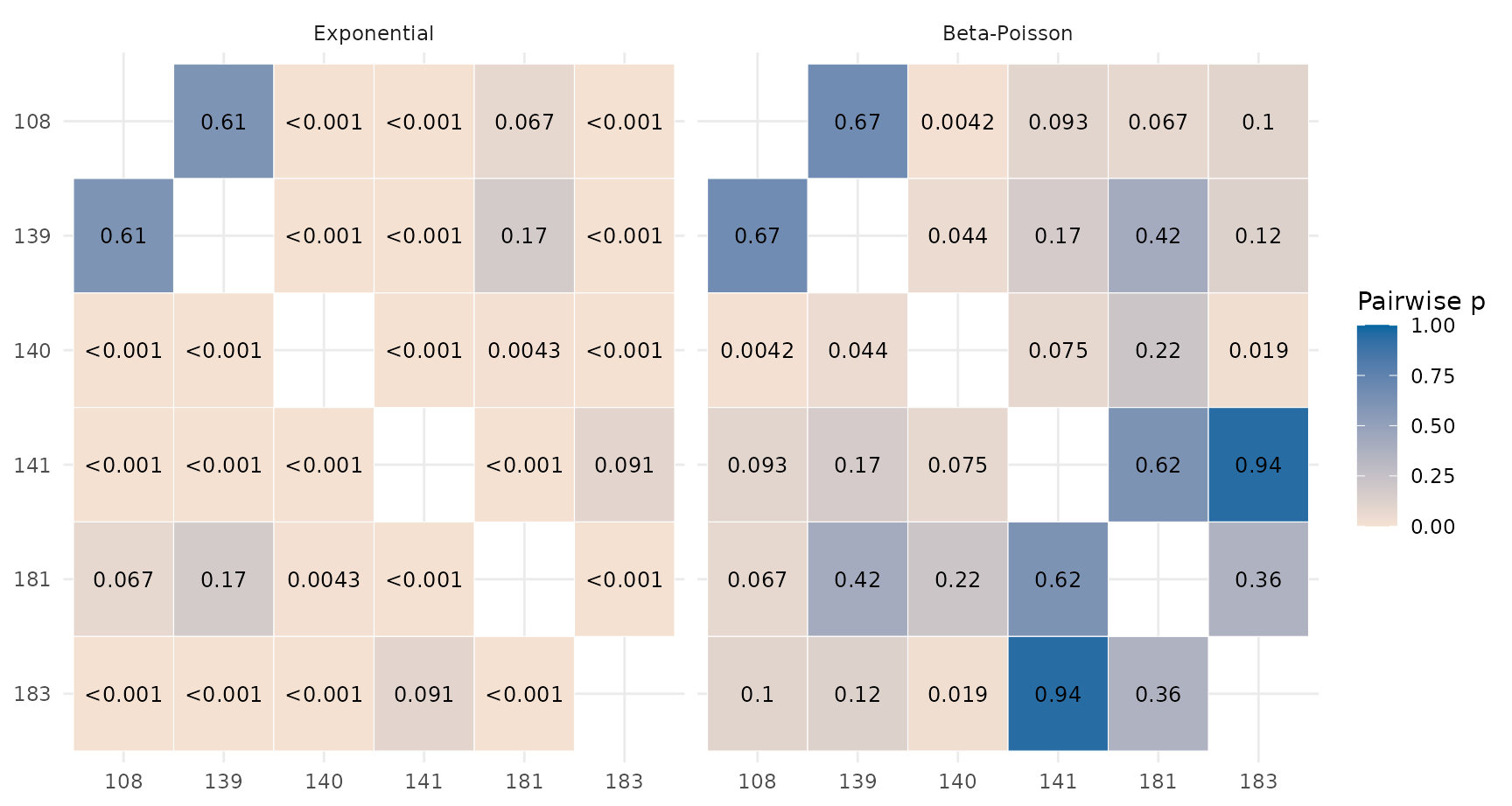
Reading one cell
Each square is one poolability test of two experiments. Pale means a small p-value: one shared curve fits clearly worse, so there is evidence the two differ. Blue means a large p-value: no evidence of a difference. The matrix is symmetric, and the diagonal is blank because an experiment always pools with itself. The grid reports no convergence flags, so read it alongside the warnings above: any cell can come from a fit that did not converge.
In the exponential panel:
- 140 (TAMU) is pale against everything (largest p = 0.0043). TAMU is far more infectious than the other isolates, and no shared curve can fit it with any of them.
- 108 and 139 (both Iowa) give p = 0.61. That looks like two studies agreeing, but see “Overlapping subjects” below.
- 181 against 139 gives p = 0.17. Experiment 181 is a different isolate (TU502) and records a different outcome (diarrhea rather than infection). It should never be pooled with infection data, yet the test does not reject it.
Why the beta-Poisson panel is bluer
The same pairs give larger p-values under beta-Poisson (mean 0.26 against 0.063 for exponential). The experiments did not become more alike; the test became weaker. The second parameter lets each curve bend to fit its own data, the test has two degrees of freedom instead of one (a higher bar to reject), and with four to eight doses per experiment the approximate beta-Poisson model is poorly determined. Beta-Poisson comparisons of small studies typically have little power.
Three mistakes to avoid
“Not rejected” is not “the same”. A p-value of 0.17 does not show that experiments 139 and 181 share a curve; it shows these data cannot tell them apart. With so few volunteers, very different experiments often pass.
Pairwise results do not chain. “A pools with B” and “B pools with C” does not mean A, B, and C share one curve. A group needs one curve for all its members, which is a stricter test than any pair.
Many tests, no correction. Each panel holds 15 tests, 30 in all. At alpha = 0.05 you would expect a “rejection” or two by chance even if every experiment were identical, and pairs can pass just as arbitrarily. None of these p-values are adjusted.
Groupings are not unique
group_datasets() turns the pairwise results into groups.
The agglomerative method (above) repeatedly merges the most compatible
pair of groups, testing each merged group as a whole, until no merge
passes; the exhaustive method searches every way of splitting the
experiments (203 ways for six) for the fewest groups that all pass.
exhaustive <- suppressWarnings(group_datasets(trials, method = "exhaustive"))
groups <- function(result, model) {
  rows <- result[result$model == model, ]
  vapply(split(rows$dataset, rows$group), paste, character(1), collapse = " + ")
}
list(
  agglomerative = list(exponential = groups(explore, "exponential"), beta_poisson = groups(explore, "beta_poisson")),
  exhaustive = list(exponential = groups(exhaustive, "exponential"), beta_poisson = groups(exhaustive, "beta_poisson"))
)
#> $agglomerative
#> $agglomerative$exponential
#>                 1                 2                 3
#> "108 + 139 + 181"             "140"       "141 + 183"
#>
#> $agglomerative$beta_poisson
#>                       1                       2
#>             "108 + 139" "140 + 141 + 181 + 183"
#>
#>
#> $exhaustive
#> $exhaustive$exponential
#>                 1                 2                 3
#> "108 + 139 + 181"             "140"       "141 + 183"
#>
#> $exhaustive$beta_poisson
#>                 1                 2
#> "108 + 141 + 183" "139 + 140 + 181"
The same data give different groupings depending on the model and the search method. Under beta-Poisson, the exhaustive search separates the two Iowa experiments, even though the heatmap shows no difference between them (p = 0.67). Several groupings pass the tests, and the search reports one of them. In both methods the TU502 diarrhea experiment (181) joins an infection group.
This is the forking-paths problem (issue #20): when the data choose the groups, a pooled curve fitted to a chosen group, and its test, are biased toward pooling. Use the exploration to sanity-check a grouping you decided on, not to choose one.
Overlapping subjects
Look at experiments 108 and 139 side by side:
overlap <- merge(
  trials[["108"]][c("dose", "positive", "negative")],
  trials[["139"]][c("dose", "positive", "negative")],
  by = "dose", suffixes = c("_108", "_139")
)
overlap
#>    dose positive_108 negative_108 positive_139 negative_139
#> 1 3e+01            1            4            2            3
#> 2 1e+02            3            5            4            4
#> 3 3e+02            2            1            2            1
#> 4 5e+02            5            1            5            1
#> 5 1e+03            2            0            2            0
#> 6 1e+04            3            0            3            0
#> 7 1e+05            1            0            1            0
#> 8 1e+06            1            0            1            0
The counts are identical at 6 of 8 doses and differ by one volunteer at the others. That strongly suggests both entries report largely the same Iowa volunteers: DuPont and colleagues (1995) reported an Iowa-isolate challenge, and Messner and colleagues (2001) analysed Iowa-isolate data from the same investigators (Chappell and Okhuysen are authors of both). The poolability test assumes independent samples, so its p-value of 0.61 says nothing here, and pooling the two would count the same people twice. Check where each experiment’s subjects came from before pooling.
Reporting
A paragraph that reports this honestly might read:
Pairwise likelihood-ratio tests (exponential model, 15 unadjusted comparisons) showed that the TAMU isolate differed from every other experiment (p < 0.01), and a test of the three isolates studied by Messner et al. (2001) rejected a common curve (p < 0.001). We therefore modelled isolates separately. Beta-Poisson comparisons had low power (two degrees of freedom, four to eight doses per study) and some fits did not converge, so we did not use them to group experiments. Experiments 108 and 139 appear to share subjects and were not pooled.
In the Shiny app
The app’s Pooling tab runs the same functions. It requires a written reason before each test, keeps a session log of every test and exploration, and marks any set chosen from an exploration, or lying within one, as data-informed in the tab, the log, and the label of pooled data sent to Fit. Its Library tab can filter experiments by strain or isolate, so a grouping can be decided before anything is tested.